Persons unfamiliar with basic elements of FTIR spectroscopy should not attempt to use this method. This method describes sampling and analytical procedures for extractive emission measurements using Fourier transform infrared (FTIR) spectroscopy. Detailed analytical procedures for interpreting infrared spectra are described in the "Protocol for the Use of Extractive Fourier Transform Infrared (FTIR) Spectrometry in Analyses of Gaseous Emissions from Stationary Sources," hereafter referred to as the "Protocol." Definitions not given in this method are given in appendix A of the Protocol. References to specific sections in the Protocol are made throughout this Method. For additional information refer to references 1 and 2, and other EPA reports, which describe the use of FTIR spectrometry in specific field measurement applications and validation tests. The sampling procedure described here is extractive. Flue gas is extracted through a heated gas transport and handling system. For some sources, sample conditioning systems may be applicable. Some examples are given in this method. Note: sample conditioning systems may be used providing the method validation requirements in Sections 9.2 and 13.0 of this method are met.

1.1 Scope and Applicability.

1.1.1 Analytes. Analytes include hazardous air pollutants (HAPs) for which EPA reference spectra have been developed. Other compounds can also be measured with this method if reference spectra are prepared according to section 4.6 of the protocol.

1.1.2 Applicability. This method applies to the analysis of vapor phase organic or inorganic compounds which absorb energy in the mid-infrared spectral region, about 400 to 4000 cm-1 (25 to 2.5 µm). This method is used to determine compound-specific concentrations in a multi-component vapor phase sample, which is contained in a closed-path gas cell. Spectra of samples are collected using double beam infrared absorption spectroscopy. A computer program is used to analyze spectra and report compound concentrations.

1.2 Method Range and Sensitivity.

Analytical range and sensitivity depend on the frequency-dependent analyte absorptivity, instrument configuration, data collection parameters, and gas stream composition. Instrument factors include: (a) spectral resolution, (b) interferometer signal averaging time, (c) detector sensitivity and response, and (d) absorption path length.

1.2.1 For any optical configuration the analytical range is between the absorbance values of about .01 (infrared transmittance relative to the background = 0.98) and 1.0 (T = 0.1). (For absorbance > 1.0 the relation between absorbance and concentration may not be linear.)

1.2.2 The concentrations associated with this absorbance range depend primarily on the cell path length and the sample temperature. An analyte absorbance greater than 1.0, can be lowered by decreasing the optical path length. Analyte absorbance increases with a longer path length. Analyte detection also depends on the presence of other species exhibiting absorbance in the same analytical region. Additionally, the estimated lower absorbance (A) limit (A = 0.01) depends on the root mean square deviation (RMSD) noise in the analytical region.

1.2.3 The concentration range of this method is determined by the choice of optical configuration.

1.2.3.1 The absorbance for a given concentration can be decreased by decreasing the path length or by diluting the sample. There is no practical upper limit to the measurement range.

1.2.3.2 The analyte absorbance for a given concentration may be increased by increasing the cell path length or (to some extent) using a higher resolution. Both modifications also cause a corresponding increased absorbance for all compounds in the sample, and a decrease in the signal throughput. For this reason the practical lower detection range (quantitation limit) usually depends on sample characteristics such as moisture content of the gas, the presence of other interferants, and losses in the sampling system.

1.3 Sensitivity.

The limit of sensitivity for an optical configuration and integration time is determined using appendix D of the Protocol: Minimum Analyte Uncertainty, (MAU). The MAU depends on the RMSD noise in an analytical region, and on the absorptivity of the analyte in the same region.

1.4 Data Quality.

Data quality shall be determined by executing Protocol pre-test procedures in appendices B to H of the protocol and post-test procedures in appendices I and J of the protocol.

1.4.1 Measurement objectives shall be established by the choice of detection limit (DLi) and analytical uncertainty (AUi) for each analyte.

1.4.2 An instrumental configuration shall be selected. An estimate of gas composition shall be made based on previous test data, data from a similar source or information gathered in a pre-test site survey. Spectral interferants shall be identified using the selected DLi and AUi and band areas from reference spectra and interferant spectra. The baseline noise of the system shall be measured in each analytical region to determine the MAU of the instrument configuration for each analyte and interferant (MIUi).

1.4.3 Data quality for the application shall be determined, in part, by measuring the RMS (root mean square) noise level in each analytical spectral region (appendix C of the Protocol). The RMS noise is defined as the RMSD of the absorbance values in an analytical region from the mean absorbance value in the region.

1.4.4 The MAU is the minimum analyte concentration for which the AUi can be maintained; if the measured analyte concentration is less than MAUi, then data quality are unacceptable.

2.0 Summary of Method.

2.1 Principle.

References 4 through 7 provide background material on infrared spectroscopy and quantitative analysis. A summary is given in this section.

2.1.1 Infrared absorption spectroscopy is performed by directing an infrared beam through a sample to a detector. The frequency-dependent infrared absorbance of the sample is measured by comparing this detector signal (single beam spectrum) to a signal obtained without a sample in the beam path (background).

2.1.2 Most molecules absorb infrared radiation and the absorbance occurs in a characteristic and reproducible pattern. The infrared spectrum measures fundamental molecular properties and a compound can be identified from its infrared spectrum alone.

2.1.3 Within constraints, there is a linear relationship between infrared absorption and compound concentration. If this frequency dependent relationship (absorptivity) is known (measured), it can be used to determine compound concentration in a sample mixture.

2.1.4 Absorptivity is measured by preparing, in the laboratory, standard samples of compounds at known concentrations and measuring the FTIR "reference spectra" of these standard samples. These "reference spectra" are then used in sample analysis: (1) compounds are detected by matching sample absorbance bands with bands in reference spectra, and (2) concentrations are measured by comparing sample band intensities with reference band intensities.

2.1.5 This method is self-validating provided that the results meet the performance requirement of the QA spike in sections 8.6.2 and 9.0 of this method, and results from a previous method validation study support the use of this method in the application.

2.2 Sampling and Analysis.

In extractive sampling a probe assembly and pump are used to extract gas from the exhaust of the affected source and transport the sample to the FTIR gas cell. Typically, the sampling apparatus is similar to that used for single-component continuous emission monitor (CEM) measurements.

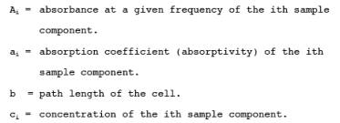
2.2.1 The digitized infrared spectrum of the sample in the FTIR gas cell is measured and stored on a computer. Absorbance band intensities in the spectrum are related to sample concentrations by what is commonly referred to as Beer's Law.

where:

2.2.2 Analyte spiking is used for quality assurance (QA). In this procedure (section 8.6.2 of this method) an analyte is spiked into the gas stream at the back end of the sample probe. Analyte concentrations in the spiked samples are compared to analyte concentrations in unspiked samples. Since the concentration of the spike is known, this procedure can be used to determine if the sampling system is removing the spiked analyte(s) from the sample stream.

2.3 Reference Spectra Availability.

Reference spectra of over 100 HAPs are available in the EPA FTIR spectral library on the EMTIC (Emission Measurement Technical Information Center) computer bulletin board service and at internet address https://info.arnold.af.mil/epa/welcome.htm. Reference spectra for HAPs, or other analytes, may also be prepared according to section 4.6 of the Protocol.

2.4 Operator Requirements.

The FTIR analyst shall be trained in setting up the instrumentation, verifying the instrument is functioning properly, and performing routine maintenance. The analyst must evaluate the initial sample spectra to determine if the sample matrix is consistent with pre-test assumptions and if the instrument configuration is suitable. The analyst must be able to modify the instrument configuration, if necessary.

2.4.1 The spectral analysis shall be supervised by someone familiar with EPA FTIR Protocol procedures.

2.4.2 A technician trained in instrumental test methods is qualified to install and operate the sampling system. This includes installing the probe and heated line assembly, operating the analyte spike system, and performing moisture and flow measurements.

3.0 Definitions.

See appendix A of the Protocol for definitions relating to infrared spectroscopy. Additional definitions are given in sections 3.1 through 3.29.

3.1 Analyte.

A compound that this method is used to measure. The term "target analyte" is also used. This method is multi-component and a number of analytes can be targeted for a test.

3.2 Reference Spectrum.

Infrared spectrum of an analyte prepared under controlled, documented, and reproducible laboratory conditions according to procedures in section 4.6 of the Protocol. A library of reference spectra is used to measure analytes in gas samples.

3.3 Standard Spectrum.

A spectrum that has been prepared from a reference spectrum through a (documented) mathematical operation. A common example is de-resolving of reference spectra to lower-resolution standard spectra (Protocol, appendix K to the addendum of this method). Standard spectra, prepared by approved, and documented, procedures can be used as reference spectra for analysis.

3.4 Concentration.

In this method concentration is expressed as a molar concentration, in ppm-meters, or in (ppm-meters)/K, where K is the absolute temperature (Kelvin). The latter units allow the direct comparison of concentrations from systems using different optical configurations or sampling temperatures.

3.5 Interferant.

A compound in the sample matrix whose infrared spectrum overlaps with part of an analyte spectrum. The most accurate analyte measurements are achieved when reference spectra of interferants are used in the quantitative analysis with the analyte reference spectra. The presence of an interferant can increase the analytical uncertainty in the measured analyte concentration.

3.6 Gas Cell.

A gas containment cell that can be evacuated. It is equipped with the optical components to pass the infrared beam through the sample to the detector. Important cell features include: path length (or range if variable), temperature range, materials of construction, and total gas volume.

3.7 Sampling System.

Equipment used to extract the sample from the test location and transport the sample gas to the FTIR analyzer. This includes sample conditioning systems.

3.8 Sample Analysis.

The process of interpreting the infrared spectra to obtain sample analyte concentrations. This process is usually automated using a software routine employing a classical least squares (cls), partial least squares (pls), or K- or P- matrix method.

3.9 One hundred percent line.

A double beam transmittance spectrum obtained by combining two background single beam spectra. Ideally, this line is equal to 100 percent transmittance (or zero absorbance) at every frequency in the spectrum. Practically, a zero absorbance line is used to measure the baseline noise in the spectrum.

3.10 Background Deviation.

A deviation from 100 percent transmittance in any region of the 100 percent line. Deviations greater than ± 5 percent in an analytical region are unacceptable (absorbance of 0.021 to -0.022). Such deviations indicate a change in the instrument throughput relative to the background single beam.

3.11 Batch Sampling.

A procedure where spectra of discreet, static samples are collected. The gas cell is filled with sample and the cell is isolated. The spectrum is collected. Finally, the cell is evacuated to prepare for the next sample.

3.12 Continuous Sampling.

A procedure where spectra are collected while sample gas is flowing through the cell at a measured rate.

3.13 Sampling resolution.

The spectral resolution used to collect sample spectra.

3.14 Truncation.

Limiting the number of interferogram data points by deleting points farthest from the center burst (zero path difference, ZPD).

3.15 Zero filling.

The addition of points to the interferogram. The position of each added point is interpolated from neighboring real data points. Zero filling adds no information to the interferogram, but affects line shapes in the absorbance spectrum (and possibly analytical results).

3.16 Reference CTS.

Calibration Transfer Standard spectra that were collected with reference spectra.

3.17 CTS Standard.

CTS spectrum produced by applying a deresolution procedure to a reference CTS.

3.18 Test CTS.

CTS spectra collected at the sampling resolution using the same optical configuration as for sample spectra. Test spectra help verify the resolution, temperature and path length of the FTIR system.

3.19 RMSD.

Root Mean Square Difference, defined in EPA FTIR Protocol, appendix A.

3.20 Sensitivity.

The noise-limited compound-dependent detection limit for the FTIR system configuration. This is estimated by the MAU. It depends on the RMSD in an analytical region of a zero absorbance line.

3.21 Quantitation Limit.

The lower limit of detection for the FTIR system configuration in the sample spectra. This is estimated by mathematically subtracting scaled reference spectra of analytes and interferences from sample spectra, then measuring the RMSD in an analytical region of the subtracted spectrum. Since the noise in subtracted sample spectra may be much greater than in a zero absorbance spectrum, the quantitation limit is generally much higher than the sensitivity. Removing spectral interferences from the sample or improving the spectral subtraction can lower the quantitation limit toward (but not below) the sensitivity.

3.22 Independent Sample.

A unique volume of sample gas; there is no mixing of gas between two consecutive independent samples. In continuous sampling two independent samples are separated by at least 5 cell volumes. The interval between independent measurements depends on the cell volume and the sample flow rate (through the cell).

3.23 Measurement.

A single spectrum of flue gas contained in the FTIR cell.

3.24 Run.

A run consists of a series of measurements. At a minimum a run includes 8 independent measurements spaced over 1 hour.

3.25 Validation.

Validation of FTIR measurements is described in sections 13.0 through 13.4 of this method. Validation is used to verify the test procedures for measuring specific analytes at a source. Validation provides proof that the method works under certain test conditions.

3.26 Validation Run.

A validation run consists of at least 24 measurements of independent samples. Half of the samples are spiked and half are not spiked. The length of the run is determined by the interval between independent samples.

3.27 Screening. Screening

is used when there is little or no available information about a source. The purpose of screening is to determine what analytes are emitted and to obtain information about important sample characteristics such as moisture, temperature, and interferences. Screening results are semi-quantitative (estimated concentrations) or qualitative (identification only). Various optical and sampling configurations may be used. Sample conditioning systems may be evaluated for their effectiveness in removing interferences. It is unnecessary to perform a complete run under any set of sampling conditions. Spiking is not necessary, but spiking can be a useful screening tool for evaluating the sampling system, especially if a reactive or soluble analyte is used for the spike.

3.28 Emissions Test.

An FTIR emissions test is performed according specific sampling and analytical procedures. These procedures, for the target analytes and the source, are based on previous screening and validation results. Emission results are quantitative. A QA spike (sections 8.6.2 and 9.2 of this method) is performed under each set of sampling conditions using a representative analyte. Flow, gas temperature and diluent data are recorded concurrently with the FTIR measurements to provide mass emission rates for detected compounds.

3.29 Surrogate.

A surrogate is a compound that is used in a QA spike procedure (section 8.6.2 of this method) to represent other compounds. The chemical and physical properties of a surrogate shall be similar to the compounds it is chosen to represent. Under given sampling conditions, usually a single sampling factor is of primary concern for measuring the target analytes: for example, the surrogate spike results can be representative for analytes that are more reactive, more soluble, have a lower absorptivity, or have a lower vapor pressure than the surrogate itself.

4.0 Interferences.

Interferences are divided into two classifications: analytical and sampling.

4.1 Analytical Interferences.

An analytical interference is a spectral feature that complicates (in extreme cases may prevent) the analysis of an analyte. Analytical interferences are classified as background or spectral interference.

4.1.1 Background Interference.

This results from a change in throughput relative to the single beam background. It is corrected by collecting a new background and proceeding with the test. In severe instances the cause must be identified and corrected. Potential causes include: (1) deposits on reflective surfaces or transmitting windows, (2) changes in detector sensitivity, (3) a change in the infrared source output, or (4) failure in the instrument electronics. In routine sampling throughput may degrade over several hours. Periodically a new background must be collected, but no other corrective action will be required.

4.1.2 Spectral Interference.

This results from the presence of interfering compound(s) (interferant) in the sample. Interferant spectral features overlap analyte spectral features. Any compound with an infrared spectrum, including analytes, can potentially be an interferant. The Protocol measures absorbance band overlap in each analytical region to determine if potential interferants shall be classified as known interferants (FTIR Protocol, section 4.9 and appendix B). Water vapor and CO2 are common spectral interferants. Both of these compounds have strong infrared spectra and are present in many sample matrices at high concentrations relative to analytes. The extent of interference depends on the (1) interferant concentration, (2) analyte concentration, and (3) the degree of band overlap. Choosing an alternate analytical region can minimize or avoid the spectral interference. For example, CO2 interferes with the analysis of the 670 cm-1 benzene band. However, benzene can also be measured near 3000 cm-1 (with less sensitivity).

4.2 Sampling System Interferences.

These prevent analytes from reaching the instrument. The analyte spike procedure is designed to measure sampling system interference, if any.

4.2.1 Temperature. A temperature that is too low causes condensation of analytes or water vapor. The materials of the sampling system and the FTIR gas cell usually set the upper limit of temperature.

4.2.2 Reactive Species. Anything that reacts with analytes. Some analytes, like formaldehyde, polymerize at lower temperatures.

4.2.3 Materials. Poor choice of material for probe, or sampling line may remove some analytes. For example, HF reacts with glass components.

4.2.4 Moisture. In addition to being a spectral interferant, condensed moisture removes soluble compounds.

5.0 Safety.

The hazards of performing this method are those associated with any stack sampling method and the same precautions shall be followed. Many HAPs are suspected carcinogens or present other serious health risks. Exposure to these compounds should be avoided in all circumstances. For instructions on the safe handling of any particular compound, refer to its material safety data sheet. When using analyte standards, always ensure that gases are properly vented and that the gas handling system is leak free. (Always perform a leak check with the system under maximum vacuum and, again, with the system at greater than ambient pressure.) Refer to section 8.2 of this method for leak check procedures. This method does not address all of the potential safety risks associated with its use. Anyone performing this method must follow safety and health practices consistent with applicable legal requirements and with prudent practice for each application.

6.0 Equipment and Supplies.

Note: Mention of trade names or specific products does not constitute endorsement by the Environmental Protection Agency.

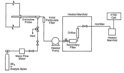
The equipment and supplies are based on the schematic of a sampling system shown in Figure 1. Either the batch or continuous sampling procedures may be used with this sampling system. Alternative sampling configurations may also be used, provided that the data quality objectives are met as determined in the post-analysis evaluation. Other equipment or supplies may be necessary, depending on the design of the sampling system or the specific target analytes.

6.1 Sampling Probe.

Glass, stainless steel, or other appropriate material of sufficient length and physical integrity to sustain heating, prevent adsorption of analytes, and to transport analytes to the infrared gas cell. Special materials or configurations may be required in some applications. For instance, high stack sample temperatures may require special steel or cooling the probe. For very high moisture sources it may be desirable to use a dilution probe.

6.2 Particulate Filters.

A glass wool plug (optional) inserted at the probe tip (for large particulate removal) and a filter (required) rated for 99 percent removal efficiency at 1-micron (e.g., Balston™) connected at the outlet of the heated probe.

6.3 Sampling Line/Heating System.

Heated (sufficient to prevent condensation) stainless steel, polytetrafluoroethane, or other material inert to the analytes.

6.4 Gas Distribution Manifold.

A heated manifold allowing the operator to control flows of gas standards and samples directly to the FTIR system or through sample conditioning systems. Usually includes heated flow meter, heated valve for selecting and sending sample to the analyzer, and a bypass vent. This is typically constructed of stainless steel tubing and fittings, and high-temperature valves.

6.5 Stainless Steel Tubing.

Type 316, appropriate diameter (e.g., 3/8 in.) and length for heated connections. Higher grade stainless may be desirable in some applications.

6.6 Calibration/Analyte Spike Assembly.

A three way valve assembly (or equivalent) to introduce analyte or surrogate spikes into the sampling system at the outlet of the probe upstream of the out-of-stack particulate filter and the FTIR analytical system.

6.7 Mass Flow Meter (MFM).

These are used for measuring analyte spike flow. The MFM shall be calibrated in the range of 0 to 5 L/min and be accurate to ± 2 percent (or better) of the flow meter span.

6.8 Gas Regulators.

Appropriate for individual gas standards.

6.9 Polytetrafluoroethane Tubing.

Diameter (e.g., 3/8 in.) and length suitable to connect cylinder regulators to gas standard manifold.

6.10 Sample Pump.

A leak-free pump (e.g., KNF™), with bypass valve, capable of producing a sample flow rate of at least 10 L/min through 100 ft of sample line. If the pump is positioned upstream of the distribution manifold and FTIR system, use a heated pump that is constructed from materials non-reactive to the analytes. If the pump is located downstream of the FTIR system, the gas cell sample pressure will be lower than ambient pressure and it must be recorded at regular intervals.

6.11 Gas Sample Manifold.

Secondary manifold to control sample flow at the inlet to the FTIR manifold. This is optional, but includes a by-pass vent and heated rotameter.

6.12 Rotameter.

A 0 to 20 L/min rotameter. This meter need not be calibrated.

6.13 FTIR Analytical System.

Spectrometer and detector, capable of measuring the analytes to the chosen detection limit. The system shall include a personal computer with compatible software allowing automated collection of spectra.

6.14 FTIR Cell Pump.

Required for the batch sampling technique, capable of evacuating the FTIR cell volume within 2 minutes. The pumping speed shall allow the operator to obtain 8 sample spectra in 1 hour.

6.15 Absolute Pressure Gauge.

Capable of measuring pressure from 0 to 1000 mmHg to within ± 2.5 mmHg (e.g., Baratron™).

6.16 Temperature Gauge.

Capable of measuring the cell temperature to within ± 2°C.

6.17 Sample Conditioning.

One option is a condenser system, which is used for moisture removal. This can be helpful in the measurement of some analytes. Other sample conditioning procedures may be devised for the removal of moisture or other interfering species.

6.17.1 The analyte spike procedure of section 9.2 of this method, the QA spike procedure of section 8.6.2 of this method, and the validation procedure of section 13 of this method demonstrate whether the sample conditioning affects analyte concentrations. Alternatively, measurements can be made with two parallel FTIR systems; one measuring conditioned sample, the other measuring unconditioned sample.

6.17.2 Another option is sample dilution. The dilution factor measurement must be documented and accounted for in the reported concentrations. An alternative to dilution is to lower the sensitivity of the FTIR system by decreasing the cell path length, or to use a short-path cell in conjunction with a long path cell to measure more than one concentration range.

7.0 Reagents and Standards.

7.1 Analyte(s) and Tracer Gas.

Obtain a certified gas cylinder mixture containing all of the analyte(s) at concentrations within ± 2 percent of the emission source levels (expressed in ppm-meter/K). If practical, the analyte standard cylinder shall also contain the tracer gas at a concentration which gives a measurable absorbance at a dilution factor of at least 10:1. Two ppm SF6 is sufficient for a path length of 22 meters at 250 °F.

7.2 Calibration Transfer Standard(s).

Select the calibration transfer standards (CTS) according to section 4.5 of the FTIR Protocol. Obtain a National Institute of Standards and Technology (NIST) traceable gravimetric standard of the CTS (± 2 percent).

7.3 Reference Spectra.

Obtain reference spectra for each analyte, interferant, surrogate, CTS, and tracer. If EPA reference spectra are not available, use reference spectra prepared according to procedures in section 4.6 of the EPA FTIR Protocol.

8.0 Sampling and Analysis Procedure.

Three types of testing can be performed: (1) screening, (2) emissions test, and (3) validation. Each is defined in section 3 of this method. Determine the purpose(s) of the FTIR test. Test requirements include: (a) AUi, DLi, overall fractional uncertainty, OFUi, maximum expected concentration (CMAXi), and tAN for each, (b) potential interferants, (c) sampling system factors, e.g., minimum absolute cell pressure, (Pmin), FTIR cell volume (VSS), estimated sample absorption pathlength, LS', estimated sample pressure, PS', TS', signal integration time (tSS), minimum instrumental line-width, MIL, fractional error, and (d) analytical regions, e.g., m = 1 to M, lower wavenumber position, FLm, center wavenumber position, FCm, and upper wavenumber position, FUm, plus interferants, upper wavenumber position of the CTS absorption band, FFUm, lower wavenumber position of the CTS absorption band, FFLm, wavenumber range FNU to FNL. If necessary, sample and acquire an initial spectrum. From analysis of this preliminary spectrum determine a suitable operational path length. Set up the sampling train as shown in Figure 1 or use an appropriate alternative configuration. Sections 8.1 through 8.11 of this method provide guidance on pre-test calculations in the EPA protocol, sampling and analytical procedures, and post-test protocol calculations.

8.1 Pretest Preparations and Evaluations.

Using the procedure in section 4.0 of the FTIR Protocol, determine the optimum sampling system configuration for measuring the target analytes. Use available information to make reasonable assumptions about moisture content and other interferences.

8.1.1 Analytes.

Select the required detection limit (DLi) and the maximum permissible analytical uncertainty (AUi) for each analyte (labeled from 1 to i). Estimate, if possible, the maximum expected concentration for each analyte, CMAXi. The expected measurement range is fixed by DLi and CMAXi for each analyte (i).

8.1.2 Potential Interferants.

List the potential interferants. This usually includes water vapor and CO2, but may also include some analytes and other compounds.

8.1.3. Optical Configuration.

Choose an optical configuration that can measure all of the analytes within the absorbance range of .01 to 1.0 (this may require more than one path length). Use Protocol sections 4.3 to 4.8 for guidance in choosing a configuration and measuring CTS.

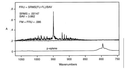
8.1.4. Fractional Reproducibility Uncertainty (FRUi).

The FRU is determined for each analyte by comparing CTS spectra taken before and after the reference spectra were measured. The EPA para-xylene reference spectra were collected on 10/31/91 and 11/01/91 with corresponding CTS spectra "cts1031a," and "cts1101b." The CTS spectra are used to estimate the reproducibility (FRU) in the system that was used to collect the references. The FRU must be < AU. Appendix E of the protocol is used to calculate the FRU from CTS spectra. Figure 2 plots results for 0.25 cm-1 CTS spectra in EPA reference library: S3 (cts1101b - cts1031a), and S4 [(cts1101b + cts1031a)/2]. The RMSD (SRMS) is calculated in the subtracted baseline, S3, in the corresponding CTS region from 850 to 1065 cm-1. The area (BAV) is calculated in the same region of the averaged CTS spectrum, S4.

8.1.5 Known Interferants.

Use appendix B of the EPA FTIR Protocol.

8.1.6 Calculate the Minimum Analyte Uncertainty, MAU

(Section 1.3 of this method discusses MAU and protocol appendix D gives the MAU procedure). The MAU for each analyte, i, and each analytical region, m, depends on the RMS noise.

8.1.7 Analytical Program.

See FTIR Protocol, section 4.10. Prepare computer program based on the chosen analytical technique. Use as input reference spectra of all target analytes and expected interferants. Reference spectra of additional compounds shall also be included in the program if their presence (even if transient) in the samples is considered possible. The program output shall be in ppm (or ppb) and shall be corrected for differences between the reference path length, LR, temperature, TR, and pressure, PR, and the conditions used for collecting the sample spectra. If sampling is performed at ambient pressure, then any pressure correction is usually small relative to corrections for path length and temperature, and may be neglected.

8.2 Leak-check.

8.2.1 Sampling System. A typical FTIR extractive sampling train is shown in Figure 1. Leak check from the probe tip to pump outlet as follows: Connect a 0– to 250-mL/min rate meter (rotameter or bubble meter) to the outlet of the pump. Close off the inlet to the probe, and record the leak rate. The leak rate shall be < 200 mL/min.

8.2.2 Analytical System Leak check. Leak check the FTIR cell under vacuum and under pressure (greater than ambient). Leak check connecting tubing and inlet manifold under

pressure.

8.2.2.1 For the evacuated sample technique, close the valve to the FTIR cell, and evacuate the absorption cell to the minimum absolute pressure Pmin. Close the valve to the pump, and determine the change in pressure •Pv after 2 minutes.

8.2.2.2 For both the evacuated sample and purging techniques, pressurize the system to about 100 mmHg above atmospheric pressure. Isolate the pump and determine the change in pressure •Pp after 2 minutes.

8.2.2.3 Measure the barometric pressure, Pb in mmHg.

8.2.2.4 Determine the percent leak volume %VL for the signal integration time tSS and for •Pmax, i.e., the larger of •Pv or •Pp, as follows:

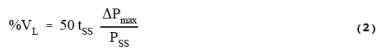
where:

50 = 100% divided by the leak-check time of 2 minutes.

8.2.2.5 Leak volumes in excess of 4 percent of the FTIR system volume VSS are unacceptable.

8.3 Detector Linearity.

Once an optical configuration is chosen, use one of the procedures of sections 8.3.1 through 8.3.3 to verify that the detector response is linear. If the detector response is not linear, decrease the aperture, or attenuate the infrared beam. After a change in the instrument configuration perform a linearity check until it is demonstrated that the detector response is linear.

8.3.1 Vary the power incident on the detector by modifying the aperture setting. Measure the background and CTS at three instrument aperture settings: (1) at the aperture setting to be used in the testing, (2) at one half this aperture and (3) at twice the proposed testing aperture. Compare the three CTS spectra. CTS band areas shall agree to within the uncertainty of the cylinder standard and the RMSD noise in the system. If test aperture is the maximum aperture, collect CTS spectrum at maximum aperture, then close the aperture to reduce the IR throughput by half. Collect a second background and CTS at the smaller aperture setting and compare the spectra again.

8.3.2 Use neutral density filters to attenuate the infrared beam. Set up the FTIR system as it will be used in the test measurements. Collect a CTS spectrum. Use a neutral density filter to attenuate the infrared beam (either immediately after the source or the interferometer) to approximately 1/2 its original intensity. Collect a second CTS spectrum. Use another filter to attenuate the infrared beam to approximately 1/4 its original intensity. Collect a third background and CTS spectrum. Compare the CTS spectra. CTS band areas shall agree to within the uncertainty of the cylinder standard and the RMSD noise in the system.

8.3.3 Observe the single beam instrument response in a frequency region where the detector response is known to be zero. Verify that the detector response is "flat" and equal to zero in these regions.

8.4 Data Storage Requirements.

All field test spectra shall be stored on a computer disk and a second backup copy must be stored on a separate disk. The stored information includes sample interferograms, processed absorbance spectra, background interferograms, CTS sample interferograms and CTS absorbance spectra. Additionally, documentation of all sample conditions, instrument settings, and test records must be recorded on hard copy or on computer medium. Table 1 gives a sample presentation of documentation.

8.5 Background Spectrum.

Evacuate the gas cell to < 5 mmHg, and fill with dry nitrogen gas to ambient pressure (or purge the cell with 10 volumes of dry nitrogen). Verify that no significant amounts of absorbing species (for example water vapor and CO2) are present. Collect a background spectrum, using a signal averaging period equal to or greater than the averaging period for the sample spectra. Assign a unique file name to the background spectrum. Store two copies of the background interferogram and processed single-beam spectrum on separate computer disks (one copy is the back-up).

8.5.1 Interference Spectra. If possible, collect spectra of known and suspected major interferences using the same optical system that will be used in the field measurements. This can be done on-site or earlier. A number of gases, e.g. CO2, SO2, CO, NH3, are readily available from cylinder gas suppliers.

8.5.2 Water vapor spectra can be prepared by the following procedure. Fill a sample tube with distilled water. Evacuate above the sample and remove dissolved gasses by alternately freezing and thawing the water while evacuating. Allow water vapor into the FTIR cell, then dilute to atmospheric pressure with nitrogen or dry air. If quantitative water spectra are required, follow the reference spectrum procedure for neat samples (protocol, section 4.6). Often, interference spectra need not be quantitative, but for best results the absorbance must be comparable to the interference absorbance in the sample spectra.

8.6 Pre-Test Calibrations

8.6.1 Calibration Transfer Standard.

Evacuate the gas cell to < 5 mmHg absolute pressure, and fill the FTIR cell to atmospheric pressure with the CTS gas. Alternatively, purge the cell with 10 cell volumes of CTS gas. (If purge is used, verify that the CTS concentration in the cell is stable by collecting two spectra 2 minutes apart as the CTS gas continues to flow. If the absorbance in the second spectrum is no greater than in the first, within the uncertainty of the gas standard, then this can be used as the CTS spectrum.) Record the spectrum.

8.6.2 QA Spike.

This procedure assumes that the method has been validated for at least some of the target analytes at the source. For emissions testing perform a QA spike. Use a certified standard, if possible, of an analyte, which has been validated at the source. One analyte standard can serve as a QA surrogate for other analytes which are less reactive or less soluble than the standard. Perform the spike procedure of section 9.2 of this method. Record spectra of at least three independent (section 3.22 of this method) spiked samples. Calculate the spiked component of the analyte concentration. If the average spiked concentration is within 0.7 to 1.3 times the expected concentration, then proceed with the testing. If applicable, apply the correction factor from the Method 301 of this appendix validation test (not the result from the QA spike).

8.7 Sampling.

If analyte concentrations vary rapidly with time, continuous sampling is preferable using the smallest cell volume, fastest sampling rate and fastest spectra collection rate possible. Continuous sampling requires the least operator intervention even without an automated sampling system. For continuous monitoring at one location over long periods, Continuous sampling is preferred. Batch sampling and continuous static sampling are used for screening and performing test runs of finite duration. Either technique is preferred for sampling several locations in a matter of days. Batch sampling gives reasonably good time resolution and ensures that each spectrum measures a discreet (and unique) sample volume. Continuous static (and continuous) sampling provides a very stable background over long periods. Like batch sampling, continuous static sampling also ensures that each spectrum measures a unique sample volume. It is essential that the leak check procedure under vacuum (section 8.2 of this method) is passed if the batch sampling procedure is used. It is essential that the leak check procedure under positive pressure is passed if the continuous static or continuous sampling procedures are used. The sampling techniques are described in sections 8.7.1 through 8.7.2 of this method.

8.7.1 Batch Sampling. Evacuate the absorbance cell to < 5 mmHg absolute pressure. Fill the cell with exhaust gas to ambient pressure, isolate the cell, and record the spectrum. Before taking the next sample, evacuate the cell until no spectral evidence of sample absorption remains. Repeat this procedure to collect eight spectra of separate samples in 1 hour.

8.7.2 Continuous Static Sampling. Purge the FTIR cell with 10 cell volumes of sample gas. Isolate the cell, collect the spectrum of the static sample and record the pressure. Before measuring the next sample, purge the cell with 10 more cell volumes of sample gas.

8.8 Sampling QA and Reporting.

8.8.1 Sample integration times shall be sufficient to achieve the required signal-to-noise ratio. Obtain an absorbance spectrum by filling the cell with N2. Measure the RMSD in each analytical region in this absorbance spectrum. Verify that the number of scans used is sufficient to achieve the target MAU.

8.8.2 Assign a unique file name to each spectrum.

8.8.3 Store two copies of sample interferograms and processed spectra on separate computer disks.

8.8.4 For each sample spectrum, document the sampling conditions, the sampling time (while the cell was being filled), the time the spectrum was recorded, the instrumental conditions (path length, temperature, pressure, resolution, signal integration time), and the spectral file name. Keep a hard copy of these data sheets.

8.9 Signal Transmittance.

While sampling, monitor the signal transmittance. If signal transmittance (relative to the background) changes by 5 percent or more (absorbance = -.02 to .02) in any analytical spectral region, obtain a new background spectrum.

8.10 Post-test CTS.

After the sampling run, record another CTS spectrum.

8.11 Post-test QA.

8.11.1 Inspect the sample spectra immediately after the run to verify that the gas matrix composition was close to the expected (assumed) gas matrix.

8.11.2 Verify that the sampling and instrumental parameters were appropriate for the conditions encountered. For example, if the moisture is much greater than anticipated, it may be necessary to use a shorter path length or dilute the sample.

8.11.3 Compare the pre- and post-test CTS spectra. The peak absorbance in pre- and post-test CTS must be ± 5 percent of the mean value. See appendix E of the FTIR Protocol.

9.0 Quality Control.

Use analyte spiking (sections 8.6.2, 9.2 and 13.0 of this method) to verify that the sampling system can transport the analytes from the probe to the FTIR system.

9.1 Spike Materials.

Use a certified standard (accurate to ± 2 percent) of the target analyte, if one can be obtained. If a certified standard cannot be obtained, follow the procedures in section 4.6.2.2 of the FTIR Protocol.

9.2 Spiking Procedure.

QA spiking (section 8.6.2 of this method) is a calibration procedure used before testing. QA spiking involves following the spike procedure of sections 9.2.1 through 9.2.3 of this method to obtain at least three spiked samples. The analyte concentrations in the spiked samples shall be compared to the expected spike concentration to verify that the sampling/analytical system is working properly. Usually, when QA spiking is used, the method has already been validated at a similar source for the analyte in question. The QA spike demonstrates that the validated sampling/analytical conditions are being duplicated. If the QA spike fails then the sampling/analytical system shall be repaired before testing proceeds. The method validation procedure (section 13.0 of this method) involves a more extensive use of the analyte spike procedure of sections 9.2.1 through 9.2.3 of this method. Spectra of at least 12 independent spiked and 12 independent unspiked samples are recorded. The concentration results are analyzed statistically to determine if there is a systematic bias in the method for measuring a particular analyte. If there is a systematic bias, within the limits allowed by Method 301 of this appendix, then a correction factor shall be applied to the analytical results. If the systematic bias is greater than the allowed limits, this method is not valid and cannot be used.

9.2.1 Introduce the spike/tracer gas at a constant flow rate of < 10 percent of the total sample flow, when possible. (Note: Use the rotameter at the end of the sampling train to estimate the required spike/tracer gas flow rate.) Use a flow device, e.g., mass flow meter (± 2 percent), to monitor the spike flow rate. Record the spike flow rate every 10 minutes.

9.2.2 Determine the response time (RT) of the system by continuously collecting spectra of the spiked effluent until the spectrum of the spiked component is constant for 5 minutes. The RT is the interval from the first measurement until the spike becomes constant. Wait for twice the duration of the RT, then collect spectra of two independent spiked gas samples. Duplicate analyses of the spiked concentration shall be within 5 percent of the mean of the two measurements.

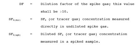
9.2.3 Calculate the dilution ratio using the tracer gas as follows:

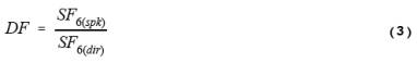
where:

10.0 Calibration and Standardization.

10.1 Signal-to-Noise Ratio (S/N).

The RMSD in the noise must be less than one tenth of the minimum analyte peak absorbance in each analytical region. For example if the minimum peak absorbance is 0.01 at the required DL, then RMSD measured over the entire analytical region must be < 0.001.

10.2 Absorbance Path length.

Verify the absorbance path length by comparing reference CTS spectra to test CTS spectra. See appendix E of the FTIR Protocol.

10.3 Instrument Resolution.

Measure the line width of appropriate test CTS band(s) to verify instrument resolution. Alternatively, compare CTS spectra to a reference CTS spectrum, if available, measured at the nominal resolution.

10.4 Apodization Function.

In transforming the sample interferograms to absorbance spectra use the same apodization function that was used in transforming the reference spectra.

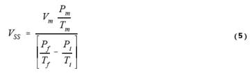
10.5 FTIR Cell Volume.

Evacuate the cell to < 5 mmHg. Measure the initial absolute temperature (Ti) and absolute pressure (Pi). Connect a wet test meter (or a calibrated dry gas meter), and slowly draw room air into the cell. Measure the meter volume (Vm), meter absolute temperature (Tm), and meter absolute pressure (Pm); and the cell final absolute temperature (Tf) and absolute pressure (Pf). Calculate the FTIR cell volume VSS, including that of the connecting tubing, as follows:

11.0 Data Analysis and Calculations.

Analyte concentrations shall be measured using reference spectra from the EPA FTIR spectral library. When EPA library spectra are not available, the procedures in section 4.6 of the Protocol shall be followed to prepare reference spectra of all the target analytes.

11.1 Spectral De-resolution.

Reference spectra can be converted to lower resolution standard spectra (section 3.3 of this method) by truncating the original reference sample and background interferograms. Appendix K of the FTIR Protocol gives specific deresolution procedures. Deresolved spectra shall be transformed using the same apodization function and level of zero filling as the sample spectra. Additionally, pre-test FTIR protocol calculations (e.g., FRU, MAU, FCU) shall be performed using the de-resolved standard spectra.

11.2 Data Analysis.

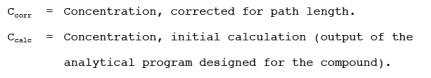
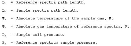
Various analytical programs are available for relating sample absorbance to a concentration standard. Calculated concentrations shall be verified by analyzing residual baselines after mathematically subtracting scaled reference spectra from the sample spectra. A full description of the data analysis and calculations is contained in the FTIR Protocol (sections 4.0, 5.0, 6.0 and appendices). Correct the calculated concentrations in the sample spectra for differences in absorption path length and temperature between the reference and sample spectra using equation 6,

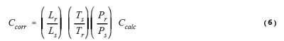
where:

12.0 Method Performance.

12.1 Spectral Quality.

Refer to the FTIR Protocol appendices for analytical requirements, evaluation of data quality, and analysis of uncertainty.

12.2 Sampling QA/QC.

The analyte spike procedure of section 9 of this method, the QA spike of section 8.6.2 of this method, and the validation procedure of section 13 of this method are used to evaluate the performance of the sampling system and to quantify sampling system effects, if any, on the measured concentrations. This method is self-validating provided that the results meet the performance requirement of the QA spike in sections 9.0 and 8.6.2 of this method and results from a previous method validation study support the use of this method in the application. Several factors can contribute to uncertainty in the measurement of spiked samples. Factors which can be controlled to provide better accuracy in the spiking procedure are listed in sections 12.2.1 through 12.2.4 of this method.

12.2.1 Flow meter. An accurate mass flow meter is accurate to ± 1 percent of its span. If a flow of 1 L/min is monitored with such a MFM, which is calibrated in the range of 0-5 L/min, the flow measurement has an uncertainty of 5 percent. This may be improved by re-calibrating the meter at the specific flow rate to be used.

12.2.2 Calibration gas. Usually the calibration standard is certified to within ± 2 percent. With reactive analytes, such as HCl, the certified accuracy in a commercially available standard may be no better than ± 5 percent.

12.2.3 Temperature. Temperature measurements of the cell shall be quite accurate. If practical, it is preferable to measure sample temperature directly, by inserting a thermocouple into the cell chamber instead of monitoring the cell outer wall temperature.

12.2.4 Pressure. Accuracy depends on the accuracy of the barometer, but fluctuations in pressure throughout a day may be as much as 2.5 percent due to weather variations.

13.0 Method Validation Procedure.

This validation procedure, which is based on EPA Method 301 (40 CFR part 63, appendix A), may be used to validate this method for the analytes in a gas matrix. Validation at one source may also apply to another type of source, if it can be shown that the exhaust gas characteristics are similar at both sources.

13.1 Analyte Spike procedure

Section 5.3 of Method 301 (40 CFR part 63, appendix A), the Analyte Spike procedure, is used with these modifications. The statistical analysis of the results follows section 6.3 of EPA Method 301. Section 3 of this method defines terms that are not defined in Method 301.

13.1.1 The analyte spike is performed dynamically. This means the spike flow is continuous and constant as spiked samples are measured.

13.1.2 The spike gas is introduced at the back of the sample probe.

13.1.3 Spiked effluent is carried through all sampling components downstream of the probe.

13.1.4 A single FTIR system (or more) may be used to collect and analyze spectra (not quadruplicate integrated sampling trains).

13.1.5 All of the validation measurements are performed sequentially in a single "run" (section 3.26 of this method).

13.1.6 The measurements analyzed statistically are each independent (section 3.22 of this method).

13.1.7 A validation data set can consist of more than 12 spiked and 12 unspiked measurements.

13.2 Batch Sampling.

The procedure in sections 13.2.1 through 13.2.2 may be used for stable processes. If process emissions are highly variable, the procedure in section

13.2.3 shall be used.

13.2.1 With a single FTIR instrument and sampling system, begin by collecting spectra of two unspiked samples. Introduce the spike flow into the sampling system and allow 10 cell volumes to purge the sampling system and FTIR cell. Collect spectra of two spiked samples. Turn off the spike and allow 10 cell volumes of unspiked sample to purge the FTIR cell. Repeat this procedure until the 24 (or more) samples are collected.

13.2.2 In batch sampling, collect spectra of 24 distinct samples. (Each distinct sample consists of filling the cell to ambient pressure after the cell has been evacuated.)

13.2.3 Alternatively, a separate probe assembly, line, and sample pump can be used for spiked sample. Verify and document that sampling conditions are the same in both the spiked and the unspiked sampling systems. This can be done by wrapping both sample lines in the same heated bundle. Keep the same flow rate in both sample lines. Measure samples in sequence in pairs. After two spiked samples are measured, evacuate the FTIR cell, and turn the manifold valve so that spiked sample flows to the FTIR cell. Allow the connecting line from the manifold to the FTIR cell to purge thoroughly (the time depends on the line length and flow rate). Collect a pair of spiked samples. Repeat the procedure until at least 24 measurements are completed.

13.3 Simultaneous Measurements With Two FTIR Systems.

If unspiked effluent concentrations of the target analyte(s) vary significantly with time, it may be desirable to perform synchronized measurements of spiked and unspiked sample. Use two FTIR systems, each with its own cell and sampling system to perform simultaneous spiked and unspiked measurements. The optical configurations shall be similar, if possible. The sampling configurations shall be the same. One sampling system and FTIR analyzer shall be used to measure spiked effluent. The other sampling system and FTIR analyzer shall be used to measure unspiked flue gas. Both systems shall use the same sampling procedure (i.e., batch or continuous).

13.3.1 If batch sampling is used, synchronize the cell evacuation, cell filling, and collection of spectra. Fill both cells at the same rate (in cell volumes per unit time).

13.3.2 If continuous sampling is used, adjust the sample flow through each gas cell so that the same number of cell volumes pass through each cell in a given time (i.e. TC1 = TC2).

13.4 Statistical Treatment.

The statistical procedure of EPA Method 301 of this appendix, section 6.3 is used to evaluate the bias and precision. For FTIR testing a validation "run" is defined as spectra of 24 independent samples, 12 of which are spiked with the analyte(s) and 12 of which are not spiked.

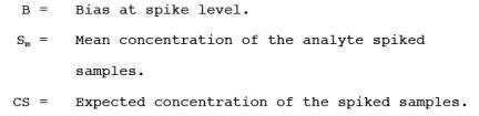
13.4.1 Bias. Determine the bias (defined by EPA Method 301 of this appendix, section 6.3.2) using equation 7:

where:

13.4.2 Correction Factor. Use section 6.3.2.2 of Method 301 of this appendix to evaluate the statistical significance of the bias. If it is determined that the bias is significant, then use section 6.3.3 of Method 301 to calculate a correction factor (CF). Analytical results of the test method are multiplied by the correction factor, if 0.7 < CF < 1.3. If is determined that the bias is significant and CF > ± 30 percent, then the test method is considered to "not valid."

13.4.3 If measurements do not pass validation, evaluate the sampling system, instrument configuration, and analytical system to determine if improper set-up or a malfunction was the cause. If so, repair the system and repeat the validation.

14.0 Pollution Prevention.

The extracted sample gas is vented outside the enclosure containing the FTIR system and gas manifold after the analysis. In typical method applications the vented sample volume is a small fraction of the source volumetric flow and its composition is identical to that emitted from the source. When analyte spiking is used, spiked pollutants are vented with the extracted sample gas. Approximately 1.6 x 10-4 to 3.2 x 10-4 lbs of a single HAP may be vented to the atmosphere in a typical validation run of 3 hours. (This assumes a molar mass of 50 to 100 g, spike rate of 1.0 L/min, and a standard concentration of 100 ppm). Minimize emissions by keeping the spike flow off when not in use.

15.0 Waste Management.

Small volumes of laboratory gas standards can be vented through a laboratory hood. Neat samples must be packed and disposed according to applicable regulations. Surplus materials may be returned to supplier for disposal.

16.0 References.

1. "Field Validation Test Using Fourier Transform Infrared (FTIR) Spectrometry To Measure Formaldehyde, Phenol and Methanol at a Wool Fiberglass Production Facility." Draft. U.S. Environmental Protection Agency Report, EPA Contract No. 68D20163, Work Assignment I-32, September 1994.

2. "FTIR Method Validation at a Coal-Fired Boiler". Prepared for U.S. Environmental Protection Agency, Research Triangle Park, NC. Publication No.: EPA-454/R95-004, NTIS No.: PB95-193199. July, 1993.

3. "Method 301 - Field Validation of Pollutant Measurement Methods from Various Waste Media," 40 CFR part 63, appendix A.

4. "Molecular Vibrations; The Theory of Infrared and Raman Vibrational Spectra," E. Bright Wilson, J. C. Decius, and P. C. Cross, Dover Publications, Inc., 1980. For a less intensive treatment of molecular rotational-vibrational spectra see, for example, "Physical Chemistry," G. M. Barrow, chapters 12, 13, and 14, McGraw Hill, Inc., 1979.

5. "Fourier Transform Infrared Spectrometry," Peter R. Griffiths and James de Haseth, Chemical Analysis, 83, 16-25,(1986), P. J. Elving, J. D. Winefordner and I. M. Kolthoff (ed.), John Wiley and Sons.

6. "Computer-Assisted Quantitative Infrared Spectroscopy," Gregory L. McClure (ed.), ASTM Special Publication 934 (ASTM), 1987.

7. "Multivariate Least-Squares Methods Applied to the Quantitative Spectral Analysis of Multicomponent Mixtures," Applied Spectroscopy, 39(10), 73-84, 1985.

Table 1. EXAMPLE PRESENTATION OF SAMPLING DOCUMENTATION.

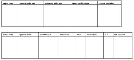
Figure 1. Extractive FTIR sampling system.

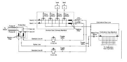
Figure 2. Fractional Reproducibility. Top: average of cts1031a and cts1101b. Bottom: Reference spectrum of p-xylene.

ADDENDUM TO TEST METHOD 320 PROTOCOL FOR THE USE OF EXTRACTIVE FOURIER TRANSFORM INFRARED (FTIR) SPECTROMETRY FOR THE ANALYSES OF GASEOUS EMISSIONS FROM STATIONARY SOURCES

1.0 INTRODUCTION

The purpose of this addendum is to set general guidelines for the use of modern FTIR spectroscopic methods for the analysis of gas samples extracted from the effluent of stationary emission sources. This addendum outlines techniques for developing and evaluating such methods and sets basic requirements for reporting and quality assurance procedures.

1.1 NOMENCLATURE

1.1.1 Appendix A to this addendum lists definitions of the symbols and terms used in this Protocol, many of which have been taken directly from American Society for Testing and Materials (ASTM) publication E 131-90a, entitled "Terminology Relating to Molecular Spectroscopy."

1.1.2 Except in the case of background spectra or where otherwise noted, the term "spectrum" refers to a double-beam spectrum in units of absorbance vs. wavenumber (cm-1).

1.1.3 The term "Study" in this addendum refers to a publication that has been subjected to EPA- or peer-review.

2.0 APPLICABILITY AND ANALYTICAL PRINCIPLE

2.1 Applicability.

This Protocol applies to the determination of compound-specific concentrations in single and multiple-component gas phase samples using double-beam absorption spectroscopy in the mid-infrared band. It does not specifically address other FTIR applications, such as single-beam spectroscopy, analysis of open-path (non-enclosed) samples, and continuous measurement techniques. If multiple spectrometers, absorption cells, or instrumental linewidths are used in such analyses, each distinct operational configuration of the system must be evaluated separately according to this Protocol.

2.2 Analytical Principle.

2.2.1 In the mid-infrared band, most molecules exhibit characteristic gas phase absorption spectra that may be recorded by FTIR systems. Such systems consist of a source of mid-infrared radiation, an interferometer, an enclosed sample cell of known absorption pathlength, an infrared detector, optical elements for the transfer of infrared radiation between components, and gas flow control and measurement components. Adjunct and integral computer systems are used for controlling the instrument, processing the signal, and for performing both Fourier transforms and quantitative analyses of spectral data.

2.2.2 The absorption spectra of pure gases and of mixtures of gases are described by a linear absorbance theory referred to as Beer's Law. Using this law, modern FTIR systems use computerized analytical programs to quantify compounds by comparing the absorption spectra of known (reference) gas samples to the absorption spectrum of the sample gas. Some standard mathematical techniques used for comparisons are classical least squares, inverse least squares, cross-correlation, factor analysis, and partial least squares. Reference A describes several of these techniques, as well as additional techniques, such as differentiation methods, linear baseline corrections, and

non-linear absorbance corrections.

3.0 GENERAL PRINCIPLES OF PROTOCOL REQUIREMENTS

The characteristics that distinguish FTIR systems from gas analyzers used in instrumental gas analysis methods (e.g., Methods 6C and 7E of appendix A to part 60 of this chapter) are: (1) Computers are necessary to obtain and analyze data; (2) chemical concentrations can be quantified using previously recorded infrared reference spectra; and (3) analytical assumptions and results, including possible effects of interfering compounds, can be evaluated after the quantitative analysis. The following general principles and requirements of this Protocol are based on these characteristics.

3.1 Verifiability and Reproducibility of Results.

Store all data and document data analysis techniques sufficient to allow an independent agent to reproduce the analytical results from the raw interferometric data.

3.2 Transfer of Reference Spectra.

To determine whether reference spectra recorded under one set of conditions (e.g., optical bench, instrumental line-width, absorption pathlength, detector performance, pressure, and temperature) can be used to analyze sample spectra taken under a different set of conditions, quantitatively compare "calibration transfer standards" (CTS) and reference spectra as described in this Protocol. (Note: The CTS may, but need not, include analytes of interest). To effect this, record the absorption spectra of the CTS (a) immediately before and immediately after recording reference spectra and (b) immediately after recording sample spectra.

3.3 Evaluation of FTIR Analyses.

The applicability, accuracy, and precision of FTIR measurements are influenced by a number of interrelated factors, which may be divided into two classes:

3.3.1 Sample-Independent Factors.

Examples are system configuration and performance (e.g., detector sensitivity and infrared source output), quality and applicability of reference absorption spectra, and type of mathematical analyses of the spectra. These factors define the fundamental limitations of FTIR measurements for a given system configuration. These limitations may be estimated from evaluations of the system before samples are available. For example, the detection limit for the absorbing compound under a given set of conditions may be estimated from the system noise level and the strength of a particular absorption band. Similarly, the accuracy of measurements may be estimated from the analysis of the reference spectra.

3.3.2 Sample-Dependent Factors.

Examples are spectral interferants (e.g., water vapor and CO2) or the overlap of spectral features of different compounds and contamination deposits on reflective surfaces or transmitting windows. To maximize the effectiveness of the mathematical techniques used in spectral analysis, identification of interferants (a standard initial step) and analysis of samples (includes effect of other analytical errors) are necessary. Thus, the Protocol requires post-analysis calculation of measurement concentration uncertainties for the detection of these potential sources of measurement error.

4.0 PRE-TEST PREPARATIONS AND EVALUATIONS

Before testing, demonstrate the suitability of FTIR spectrometry for the desired application according to the procedures of this section.

4.1 Identify Test Requirements.

Identify and record the test requirements described in sections 4.1.1 through 4.1.4 of this addendum. These values set the desired or required goals of the proposed analysis; the description of methods for determining whether these goals are actually met during the analysis comprises the majority of this Protocol.

4.1.1 Analytes (specific chemical species) of interest. Label the analytes from i = 1 to I.

4.1.2 Analytical uncertainty limit (AUi). The AUi is the maximum permissible fractional uncertainty of analysis for the ith analyte concentration, expressed as a fraction of the analyte concentration in the sample.

4.1.3 Required detection limit for each analyte (DLi, ppm). The detection limit is the lowest concentration of an analyte for which its overall fractional uncertainty (OFUi) is required to be less than its analytical uncertainty limit (AUi).

4.1.4 Maximum expected concentration of each analyte (CMAXi, ppm).

4.2 Identify Potential Interferants.

Considering the chemistry of the process or results of previous studies, identify potential interferants, i.e., the major effluent constituents and any relatively minor effluent constituents that possess either strong absorption characteristics or strong structural similarities to any analyte of interest. Label them 1 through Nj, where the subscript "j" pertains to potential interferants. Estimate the concentrations of these compounds in the effluent (CPOTj, ppm).

4.3 Select and Evaluate the Sampling System.

Considering the source, e.g., temperature and pressure profiles, moisture content, analyte characteristics, and particulate concentration), select the equipment for extracting gas samples. Recommended are a particulate filter, heating system to maintain sample temperature above the dew point for all sample constituents at all points within the sampling system (including the filter), and sample conditioning system (e.g., coolers, water-permeable membranes that remove water or other compounds from the sample, and dilution devices) to remove spectral interferants or to protect the sampling and analytical components. Determine the minimum absolute sample system pressure (Pmin, mmHg) and the infrared absorption cell volume (VSS, liter). Select the techniques and/or equipment for the measurement of sample pressures and temperatures.

4.4 Select Spectroscopic System.

Select a spectroscopic configuration for the application. Approximate the absorption pathlength (LS', meter), sample pressure (PS', kPa), absolute sample temperature TS', and signal integration period (tSS, seconds) for the analysis. Specify the nominal minimum instrumental linewidth (MIL) of the system. Verify that the fractional error at the approximate values PS' and TS' is less than one half the smallest value AUi (see section 4.1.2 of this addendum).

4.5 Select Calibration Transfer Standards (CTS's).

Select CTS's that meet the criteria listed in sections 4.5.1, 4.5.2, and 4.5.3 of this addendum.

Note: It may be necessary to choose preliminary analytical regions (see section 4.7 of this addendum), identify the minimum analyte line-widths, or estimate the system noise level (see section 4.12 of this addendum) before selecting the CTS. More than one compound may be needed to meet the criteria; if so, obtain separate cylinders for each compound.

4.5.1 The central wavenumber position of each analytical region shall lie within 25 percent of the wavenumber position of at least one CTS absorption band.

4.5.2 The absorption bands in section 4.5.1 of this addendum shall exhibit peak absorbances greater than ten times the value RMSEST (see section 4.12 of this addendum) but less than 1.5 absorbance units.

4.5.3 At least one absorption CTS band within the operating range of the FTIR instrument shall have an instrument-independent line-width no greater than the narrowest analyte absorption band. Perform and document measurements or cite Studies to determine analyte and CTS compound line-widths.

4.5.4 For each analytical region, specify the upper and lower wavenumber positions (FFUm and FFLm, respectively) that bracket the CTS absorption band or bands for the associated analytical region. Specify the wavenumber range, FNU to FNL, containing the absorption band that meets the criterion of section 4.5.3 of this addendum.

4.5.5 Associate, whenever possible, a single set of CTS gas cylinders with a set of reference spectra. Replacement CTS gas cylinders shall contain the same compounds at concentrations within 5 percent of that of the original CTS cylinders; the entire absorption spectra (not individual spectral segments) of the replacement gas shall be scaled by a factor between 0.95 and 1.05 to match the original CTS spectra.

4.6 Prepare Reference Spectra.

Note: Reference spectra are available in a permanent soft copy from the EPA spectral library on the EMTIC (Emission Measurement Technical Information Center) computer bulletin board; they may be used if applicable.

4.6.1 Select the reference absorption pathlength (LR) of the cell.

4.6.2 Obtain or prepare a set of chemical standards for each analyte, potential and known spectral interferants, and CTS. Select the concentrations of the chemical standards to correspond to the top of the desired range.

4.6.2.1 Commercially-Prepared Chemical Standards. Chemical standards for many compounds may be obtained from independent sources, such as a specialty gas manufacturer, chemical company, or commercial laboratory. These standards (accurate to within ±2 percent) shall be prepared according to EPA Traceability Protocol (see Reference D) or shall be traceable to NIST standards. Obtain from the supplier an estimate of the stability of the analyte concentration. Obtain and follow all of the supplier's recommendations for recertifying the analyte concentration.

4.6.2.2 Self-Prepared Chemical Standards. Chemical standards may be prepared by diluting certified commercially prepared chemical gases or pure analytes with ultra-pure carrier (UPC) grade nitrogen according to the barometric and volumetric techniques generally described in Reference A, section A4.6.

4.6.3 Record a set of the absorption spectra of the CTS {R1}, then a set of the reference spectra at two or more concentrations in duplicate over the desired range (the top of the range must be less than 10 times that of the bottom), followed by a second set of CTS spectra {R2}. (If self-prepared standards are used, see section 4.6.5 of this addendum before disposing of any of the standards.) The maximum accepted standard concentration-pathlength product (ASCPP) for each compound shall be higher than the maximum estimated concentration-pathlength products for both analytes and known interferants in the effluent gas. For each analyte, the minimum ASCPP shall be no greater than ten times the concentration-pathlength product of that analyte at its required detection limit.

4.6.4 Permanently store the background and interferograms in digitized form. Document details of the mathematical process for generating the spectra from these interferograms. Record the sample pressure (PR), sample temperature (TR), reference absorption pathlength (LR), and interferogram signal integration period (tSR). Signal integration periods for the background interferograms shall be >tSR. Values of PR, LR, and tSR shall not deviate by more than ±1 percent from the time of recording {R1} to that of recording {R2}.

4.6.5 If self-prepared chemical standards are employed and spectra of only two concentrations are recorded for one or more compounds, verify the accuracy of the dilution technique by analyzing the prepared standards for those compounds with a secondary (non-FTIR) technique in accordance with sections 4.6.5.1 through 4.6.5.4 of this addendum.

4.6.5.1 Record the response of the secondary technique to each of the four standards prepared.

4.6.5.2 Perform a linear regression of the response values (dependant variable) versus the accepted standard concentration (ASC) values (independent variable), with the regression constrained to pass through the zero-response, zero ASC point.

4.6.5.3 Calculate the average fractional difference between the actual response values and the regression predicted values (those calculated from the regression line using the four ASC values as the independent variable).

4.6.5.4 If the average fractional difference value calculated in section 4.6.5.3 of this addendum is larger for any compound than the corresponding AUi, the dilution technique is not sufficiently accurate and the reference spectra prepared are not valid for the analysis.

4.7 Select Analytical Regions.

Using the general considerations in section 7 of Reference A and the spectral characteristics of the analytes and interferants, select the analytical regions for the application. Label them m = 1 to M. Specify the lower, center and upper wavenumber positions of each analytical region (FLm, FCm, and FUm, respectively). Specify the analytes and interferants which exhibit absorption in each region.

4.8 Determine Fractional Reproducibility Uncertainties.

Using appendix E of this addendum, calculate the fractional reproducibility uncertainty for each analyte (FRUi) from a comparison of {R1} and {R2}. If FRUi > AUi for any analyte, the reference spectra generated in accordance with section 4.6 of this addendum are not valid for the application.

4.9 Identify Known Interferants.

Using appendix B of this addendum, determine which potential interferants affect the analyte concentration determinations. Relabel these potential interferant as "known" interferants, and designate these compounds from k = 1 to K. Appendix B to this addendum also provides criteria for determining whether the selected analytical regions are suitable.

4.10 Prepare Computerized Analytical Programs.

4.10.1 Choose or devise mathematical techniques (e.g, classical least squares, inverse least squares, cross-correlation, and factor analysis) based on equation 4 of Reference A that are appropriate for analyzing spectral data by comparison with reference spectra.

4.10.2 Following the general recommendations of Reference A, prepare a computer program or set of programs that analyzes all of the analytes and known interferants, based on the selected analytical regions (section 4.7 of this addendum) and the prepared reference spectra (section 4.6 of this addendum). Specify the baseline correction technique (e.g., determining the slope and intercept of a linear baseline contribution in each analytical region) for each analytical region, including all relevant wavenumber positions.

4.10.3 Use programs that provide as output [at the reference absorption pathlength (LR), reference gas temperature (TR), and reference gas pressure (PR)] the analyte concentrations, the known interferant concentrations, and the baseline slope and intercept values. If the sample absorption pathlength (LS), sample gas temperature (TS), or sample gas pressure (PS) during the actual sample analyses differ from LR, TR, and PR, use a program or set of programs that applies multiplicative corrections to the derived concentrations to account for these variations, and that provides as output both the corrected and uncorrected values. Include in the report of the analysis (see section 7.0 of this addendum) the details of any transformations applied to the original reference spectra (e.g., differentiation), in such a fashion that all analytical results may be verified by an independent agent from the reference spectra and data spectra alone.

4.11 Determine the Fractional Calibration Uncertainty.

Calculate the fractional calibration uncertainty for each analyte (FCUi) according to appendix F of this addendum, and compare these values to the fractional uncertainty limits (AUi; see section 4.1.2 of this addendum). If FCUi > AUi, either the reference spectra or analytical programs for that analyte are unsuitable.

4.12 Verify System Configuration Suitability.

Using appendix C of this addendum, measure or obtain estimates of the noise level (RMSEST, absorbance) of the FTIR system. Alternatively, construct the complete spectrometer system and determine the values RMSSm using appendix G of this addendum. Estimate the minimum measurement uncertainty for each analyte (MAUi, ppm) and known interferant (MIUk, ppm) using appendix D of this addendum. Verify that (a) MAUi < (AUi)(DLi), FRUi < AUi, and FCUi < AUi for each analyte and that (b) the CTS chosen meets the requirements listed in sections 4.5.1 through 4.5.5 of this addendum.

5.0 SAMPLING AND ANALYSIS PROCEDURE

5.1 Analysis System Assembly and Leak-Test.

Assemble the analysis system. Allow sufficient time for all system components to reach the desired temperature. Then, determine the leak-rate (LR) and leak volume (VL), where VL = LR tSS. Leak volumes shall be #4 percent of VSS.

5.2 Verify Instrumental Performance.

Measure the noise level of the system in each analytical region using the procedure of appendix G of this addendum. If any noise level is higher than that estimated for the system in section 4.12 of this addendum, repeat the calculations of appendix D of this addendum and verify that the requirements of section 4.12 of this addendum are met; if they are not, adjust or repair the instrument and repeat this section.

5.3 Determine the Sample Absorption Pathlength.

Record a background spectrum. Then, fill the absorption cell with CTS at the pressure PR and record a set of CTS spectra {R3}. Store the background and unscaled CTS single beam interferograms and spectra. Using appendix H of this addendum, calculate the sample absorption pathlength (LS) for each analytical region. The values LS shall not differ from the approximated sample pathlength LS' (see section 4.4 of this addendum) by more than 5 percent.

5.4 Record Sample Spectrum.

Connect the sample line to the source. Either evacuate the absorption cell to an absolute pressure below 5 mmHg before extracting a sample from the effluent stream into the absorption cell, or pump at least ten cell volumes of sample through the cell before obtaining a sample. Record the sample pressure PS. Generate the absorbance spectrum of the sample. Store the background and sample single beam interferograms, and document the process by which the absorbance spectra are generated from these data. (If necessary, apply the spectral transformations developed in section 5.6.2 of this addendum). The resulting sample spectrum is referred to below as SS.

Note: Multiple sample spectra may be recorded according to the procedures of section 5.4 of this addendum before performing sections 5.5 and 5.6 of this addendum.

5.5 Quantify Analyte Concentrations.

Calculate the unscaled analyte concentrations RUAi and unscaled interferant concentrations RUIK using the programs developed in section 4 of this addendum. To correct for pathlength and pressure variations between the reference and sample spectra, calculate the scaling factor, RLPS using equation A.1,

Calculate the final analyte and interferant concentrations RSAi and RSIk using equations A.2 and A.3,

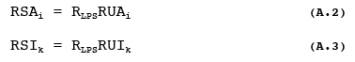
5.6 Determine Fractional Analysis Uncertainty.

Fill the absorption cell with CTS at the pressure PS. Record a set of CTS spectra {R4}. Store the background and CTS single beam interferograms. Using appendix H of this addendum, calculate the fractional analysis uncertainty (FAU) for each analytical region. If the FAU indicated for any analytical region is greater than the required accuracy requirements determined in sections 4.1.1 through 4.1.4 of this addendum, then comparisons to previously recorded reference spectra are invalid in that analytical region, and the analyst shall perform one or both of the procedures of sections 5.6.1 through 5.6.2 of this addendum.

5.6.1 Perform instrumental checks and adjust the instrument to restore its performance to acceptable levels. If adjustments are made, repeat sections 5.3, 5.4 (except for the recording of a sample spectrum), and 5.5 of this addendum to demonstrate that acceptable uncertainties are obtained in all analytical regions.

5.6.2 Apply appropriate mathematical transformations (e.g., frequency shifting, zero-filling, apodization, smoothing) to the spectra (or to the interferograms upon which the spectra are based) generated during the performance of the procedures of section 5.3 of this addendum. Document these transformations and their reproducibility. Do not apply multiplicative scaling of the spectra, or any set of transformations that is mathematically equivalent to multiplicative scaling. Different transformations may be applied to different analytical regions. Frequency shifts shall be less than one-half the minimum instrumental line-width, and must be applied to all spectral data points in an analytical region. The mathematical transformations may be retained for the analysis if they are also applied to the appropriate analytical regions of all sample spectra recorded, and if all original sample spectra are digitally stored. Repeat sections 5.3, 5.4 (except the recording of a sample spectrum), and 5.5 of this addendum to demonstrate that these transformations lead to acceptable calculated concentration uncertainties in all analytical regions.

6.0 POST-ANALYSIS EVALUATIONS

Estimate the overall accuracy of the analyses performed in accordance with sections 5.1 through 5.6 of this addendum using the procedures of sections 6.1 through 6.3 of this addendum.

6.1 Qualitatively Confirm the Assumed Matrix.

Examine each analytical region of the sample spectrum for spectral evidence of unexpected or unidentified interferants. If found, identify the interfering compounds (see Reference C for guidance) and add them to the list of known interferants. Repeat the procedures of section 4 of this addendum to include the interferants in the uncertainty calculations and analysis procedures. Verify that the MAU and FCU values do not increase beyond acceptable levels for the application requirements. Re-calculate the analyte concentrations (section 5.5 of this addendum) in the affected analytical regions.

6.2 Quantitatively Evaluate Fractional Model Uncertainty (FMU).

Perform the procedures of either section 6.2.1 or 6.2.2 of this addendum:

6.2.1 Using appendix I of this addendum, determine the fractional model error (FMU) for each analyte.

6.2.2 Provide statistically determined uncertainties FMU for each analyte which are equivalent to two standard deviations at the 95 percent confidence level. Such determinations, if employed, must be based on mathematical examinations of the pertinent sample spectra (not the reference spectra alone). Include in the report of the analysis (see section 7.0 of this addendum) a complete description of the determination of the concentration uncertainties.

6.3 Estimate Overall Concentration Uncertainty (OCU).

Using appendix J of this addendum, determine the overall concentration uncertainty (OCU) for each analyte. If the OCU is larger than the required accuracy for any analyte, repeat sections 4 and 6 of this addendum.

7.0 REPORTING REQUIREMENTS

[Documentation pertaining to virtually all the procedures of sections 4, 5, and 6 will be required. Software copies of reference spectra and sample spectra will be retained for some minimum time following the actual testing.]

8.0 REFERENCES

A) Standard Practices for General Techniques of Infrared Quantitative Analysis (American Society for Testing and Materials, Designation E 168-88).

B) The Coblentz Society Specifications for Evaluation of Research Quality Analytical Infrared Reference Spectra (Class II); Anal. Chemistry 47, 945A (1975); Appl. Spectroscopy 444, pp. 211-215, 1990.

C) Standard Practices for General Techniques for Qualitative Infrared Analysis, American Society for Testing and Materials, Designation E 1252-88.

D) "EPA Traceability Protocol for Assay and Certification of Gaseous Calibration Standards," U.S. Environmental Protection Agency Publication No. EPA/600/R-93/224, December 1993.

APPENDIX A to Addendum to Method 320

DEFINITIONS OF TERMS AND SYMBOLS

A.1 Definitions of Terms.

All terms used in this method that are not defined below have the meaning given to them in the CAA and in subpart A of this part.

Absorption band means a contiguous wavenumber region of a spectrum (equivalently, a contiguous set of absorbance spectrum data points) in which the absorbance passes through a maximum or a series of maxima.

Absorption pathlength means the distance in a spectrophotometer, measured in the direction of propagation of the beam of radiant energy, between the surface of the specimen on which the radiant energy is incident and the surface of the specimen from which it is emergent.

Analytical region means a contiguous wavenumber region (equivalently, a contiguous set of absorbance spectrum data points) used in the quantitative analysis for one or more analytes.

Note: The quantitative result for a single analyte may be based on data from more than one analytical region. Apodization means modification of the ILS function by multiplying the interferogram by a weighing function whose magnitude varies with retardation.

Background spectrum means the single beam spectrum obtained with all system components without sample present.

Baseline means any line drawn on an absorption spectrum to establish a reference point that represents a function of the radiant power incident on a sample at a given wavelength.

Beers's law means the direct proportionality of the absorbance of a compound in a homogeneous sample to its concentration.

Calibration transfer standard (CTS) gas means a gas standard of a compound used to achieve and/or demonstrate suitable quantitative agreement between sample spectra and the reference spectra; see section 4.5.1 of this addendum.

Compound means a substance possessing a distinct, unique molecular structure.

Concentration (c) means the quantity of a compound contained in a unit quantity of sample. The unit "ppm" (number, or mole, basis) is recommended.

Concentration-pathlength product means the mathematical product of concentration of the species and absorption pathlength. For reference spectra, this is a known quantity; for sample spectra, it is the quantity directly determined from Beer's law. The units "centimeters-ppm" or "meters-ppm" are recommended.

Derivative absorption spectrum means a plot of rate of change of absorbance or of any function of absorbance with respect to wavelength or any function of wavelength.

Double beam spectrum means a transmission or absorbance spectrum derived by dividing the sample single beam spectrum by the background spectrum.

Note: The term "double-beam" is used elsewhere to denote a spectrum in which the sample and background interferograms are collected simultaneously along physically distinct absorption paths. Here, the term denotes a spectrum in which the sample and background interferograms are collected at different times along the same absorption path.

Fast Fourier transform (FFT) means a method of speeding up the computation of a discrete FT by factoring the data into sparse matrices containing mostly zeros.

Flyback means interferometer motion during which no data are recorded.

Fourier transform (FT) means the mathematical process for converting an amplitude-time spectrum to an amplitude frequency spectrum, or vice versa.

Fourier transform infrared (FTIR) spectrometer means an analytical system that employs a source of mid-infrared radiation, an interferometer, an enclosed sample cell of known absorption pathlength, an infrared detector, optical elements that transfer infrared radiation between components, and a computer system. The time-domain detector response (interferogram) is processed by a Fourier transform to yield a representation of the detector response vs. infrared frequency.

Note: When FTIR spectrometers are interfaced with other instruments, a slash should be used to denote the interface; e.g., GC/FTIR; HPCL/FTIR, and the use of FTIR should be explicit; i.e., FTIR not IR.

Frequency, v means the number of cycles per unit time.

Infrared means the portion of the electromagnetic spectrum containing wavelengths from approximately 0.78 to 800 microns.

Interferogram, I(•) means record of the modulated component of the interference signal measured as a function of retardation by the detector.

Interferometer means device that divides a beam of radiant energy into two or more paths, generates an optical path difference between the beams, and recombines them in order to produce repetitive interference maxima and minima as the optical retardation is varied.

Linewidth means the full width at half maximum of an absorption band in units of wavenumbers (cm-1). Mid-infrared means the region of the electromagnetic spectrum from approximately 400 to 5000 cm-1.

Reference spectra means absorption spectra of gases with known chemical compositions, recorded at a known absorption pathlength, which are used in the quantitative analysis of gas samples.

Retardation, • means optical path difference between two beams in an interferometer; also known as "optical path difference" or "optical retardation."

Scan means digital representation of the detector output obtained during one complete motion of the interferometer's moving assembly or assemblies.

Scaling means application of a multiplicative factor to the absorbance values in a spectrum.

Single beam spectrum means Fourier-transformed interferogram, representing the detector response vs. wavenumber.

Note: The term "single-beam" is used elsewhere to denote any spectrum in which the sample and background interferograms are recorded on the same physical absorption path; such usage differentiates such spectra from those generated using interferograms recorded along two physically distinct absorption paths (see "double-beam spectrum" above). Here, the term applies (for example) to the two spectra used directly in the calculation of transmission and absorbance spectra of a sample.

Standard reference material means a reference material, the composition or properties of which are certified by a recognized standardizing agency or group.

Note: The equivalent ISO term is "certified reference material."

Transmittance, T means the ratio of radiant power transmitted by the sample to the radiant power incident on the sample. Estimated in FTIR spectroscopy by forming the ratio of the single-beam sample and background spectra.

Wavenumber, v means the number of waves per unit length.

Note: The usual unit of wavenumber is the reciprocal centimeter, cm-1. The wavenumber is the reciprocal of the wavelength, 8, when 8 is expressed in centimeters.

Zero-filling means the addition of zero-valued points to the end of a measured interferogram.

Note: Performing the FT of a zero-filled interferogram results in correctly interpolated points in the computed spectrum.

A.2 Definitions of Mathematical Symbols.

The symbols used in equations in this protocol are defined as follows:

(1) A, absorbance = the logarithm to the base 10 of the reciprocal of the transmittance (T).

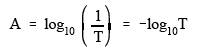
(2) AAIim = band area of the ith analyte in the mth analytical region, at the concentration (CLi) corresponding to the product of its required detection limit (DLi) and analytical uncertainty limit (AUi) .

(3) AAVim = average absorbance of the ith analyte in the mth analytical region, at the concentration (CLi) corresponding to the product of its required detection limit (DLi) and analytical uncertainty limit (AUi) .

(4) ASC, accepted standard concentration = the concentration value assigned to a chemical standard.

(5) ASCPP, accepted standard concentration-pathlength product = for a chemical standard, the product of the ASC and the sample absorption pathlength. The units "centimeters-ppm" or "meters-ppm" are recommended.

(6) AUi, analytical uncertainty limit = the maximum permissible fractional uncertainty of analysis for the ith analyte concentration, expressed as a fraction of the analyte concentration determined in the analysis.

(7) AVTm = average estimated total absorbance in the mth analytical region.

(8) CKWNk = estimated concentration of the kth known interferant.

(9) CMAXi = estimated maximum concentration of the ith analyte.

(10) CPOTj = estimated concentration of the jth potential interferant.

(11) DLi, required detection limit = for the ith analyte, the lowest concentration of the analyte for which its overall fractional uncertainty (OFUi) is required to be less than the analytical uncertainty limit (AUi).

(12) FCm = center wavenumber position of the mth analytical region.

(13) FAUi, fractional analytical uncertainty = calculated uncertainty in the measured concentration of the ith analyte because of errors in the mathematical comparison of reference and sample spectra.

(14) FCUi, fractional calibration uncertainty = calculated uncertainty in the measured concentration of the ith analyte because of errors in Beer's law modeling of the reference spectra concentrations.

(15) FFLm = lower wavenumber position of the CTS absorption band associated with the mth analytical region.

(16) FFUm = upper wavenumber position of the CTS absorption band associated with the mth analytical region.

(17) FLm = lower wavenumber position of the mth analytical region.

(18) FMUi, fractional model uncertainty = calculated uncertainty in the measured concentration of the ith analyte because of errors in the absorption model employed.

(19) FNL = lower wavenumber position of the CTS spectrum containing an absorption band at least as narrow as the analyte absorption bands.

(20) FNU = upper wavenumber position of the CTS spectrum containing an absorption band at least as narrow as the analyte absorption bands.

(21) FRUi, fractional reproducibility uncertainty = calculated uncertainty in the measured concentration of the ith analyte because of errors in the reproducibility of spectra from the FTIR system.

(22) FUm = upper wavenumber position of the mth analytical region.

(23) IAIjm = band area of the jth potential interferant in the mth analytical region, at its expected concentration (CPOTj).

(24) IAVim = average absorbance of the ith analyte in the mth analytical region, at its expected concentration (CPOTj).

(25) ISCi or k, indicated standard concentration = the concentration from the computerized analytical program for a single-compound reference spectrum for the ith analyte or kth known interferant.

(26) kPa = kilo-Pascal (see Pascal).

(27) LS' = estimated sample absorption pathlength.

(28) LR = reference absorption pathlength.

(29) LS = actual sample absorption pathlength.

(30) MAUi = mean of the MAUim over the appropriate analytical regions.

(31) MAUim, minimum analyte uncertainty = the calculated minimum concentration for which the analytical uncertainty limit (AUi) in the measurement of the ith analyte, based on spectral data in the mth analytical region, can be maintained.

(32) MIUj = mean of the MIUjm over the appropriate analytical regions.

(33) MIUjm, minimum interferant uncertainty = the calculated minimum concentration for which the analytical uncertainty limit CPOTj/20 in the measurement of the jth interferant, based on spectral data in the mth analytical region, can be maintained.

(34) MIL, minimum instrumental line-width = the minimum line-width from the FTIR system, in wavenumbers.

Note: The MIL of a system may be determined by observing an absorption band known (through higher resolution examinations) to be narrower than indicated by the system. The MIL is fundamentally limited by the retardation of the interferometer, but is also affected by other operational parameters (e.g., the choice of apodization).

(35) Ni = number of analytes.

(36) Nj = number of potential interferants.

(37) Nk = number of known interferants.

(38) Nscan = the number of scans averaged to obtain an

interferogram.

(39) OFUi = the overall fractional uncertainty in an analyte concentration determined in the analysis (OFUi = MAX{FRUi, FCUi, FAUi, FMUi}).

(40) Pascal (Pa) = metric unit of static pressure, equal to one Newton per square meter; one atmosphere is equal to 101,325 Pa; 1/760 atmosphere (one Torr, or one millimeter Hg) is equal to 133.322 Pa.

(41) Pmin = minimum pressure of the sampling system during the sampling procedure.

(42) PS' = estimated sample pressure.

(43) PR = reference pressure.

(44) PS = actual sample pressure.

(45) RMSSm = measured noise level of the FTIR system in the mth analytical region.

(46) RMSD, root mean square difference = a measure of accuracy determined by the following equation:

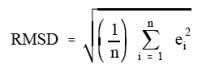
where:

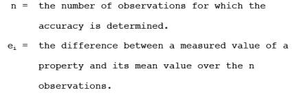
Note: The RMSD value "between a set of n contiguous absorbance values (Ai) and the mean of the values" (AM) is defined as

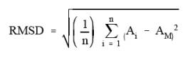
(47) RSAi = the (calculated) final concentration of the ith analyte.

(48) RSIk = the (calculated) final concentration of the kth known interferant.

(49) tscan, scan time = time used to acquire a single scan, not including flyback.

(50) tS, signal integration period = the period of time over which an interferogram is averaged by addition and scaling of individual scans. In terms of the number of scans Nscan and scan time tscan, tS = Nscantscan.

(51) tSR = signal integration period used in recording reference spectra.

(52) tSS = signal integration period used in recording sample spectra.

(53) TR = absolute temperature of gases used in recording reference spectra.

(54) TS = absolute temperature of sample gas as sample spectra are recorded.

(55) TP, Throughput = manufacturer's estimate of the fraction of the total infrared power transmitted by the absorption cell and transfer optics from the interferometer to the detector.

(56) VSS = volume of the infrared absorption cell, including parts of attached tubing.

(57) Wik = weight used to average over analytical regions k for quantities related to the analyte i; see appendix D of this addendum.

APPENDIX B TO ADDENDUM TO METHOD 320

IDENTIFYING SPECTRAL INTERFERANTS

B.1 General

B.1.1 Assume a fixed absorption pathlength equal to the value LS'.

B.1.2 Use band area calculations to compare the relative absorption strengths of the analytes and potential interferants. In the mth analytical region (FLm to FUm), use either rectangular or trapezoidal approximations to determine the band areas described below (see Reference A, sections A.3.1 through A.3.3). Document any baseline corrections applied to the spectra.

B.1.3 Use the average total absorbance of the analytes and potential interferants in each analytical region to determine whether the analytical region is suitable for analyte concentration determinations.

Note: The average absorbance in an analytical region is the band area divided by the width of the analytical region in wavenumbers. The average total absorbance in an analytical region is the sum of the average absorbances of all analytes and potential interferants.

B.2 Calculations

B.2.1 Prepare spectral representations of each analyte at the concentration CLi = (DLi)(AUi), where DLi is the required detection limit and AUi is the maximum permissible analytical uncertainty. For the mth analytical region, calculate the band area (AAIim) and average absorbance (AAVim) from these scaled analyte spectra.

B.2.2 Prepare spectral representations of each potential interferant at its expected concentration (CPOTj). For the mth analytical region, calculate the band area (IAIjm) and average absorbance (IAVjm) from these scaled potential interferant spectra.

B.2.3 Repeat the calculation for each analytical region, and record the band area results in matrix form as indicated in Figure B.1.

B.2.4 If the band area of any potential interferant in an analytical region is greater than the one-half the band area of any analyte (i.e., IAIjm > 0.5 AAIim for any pair ij and any m), classify the potential interferant as a known interferant. Label the known interferants k = 1 to K. Record the results in matrix form as indicated in Figure B.2.

B.2.5 Calculate the average total absorbance (AVTm) for each analytical region and record the values in the last row of the matrix described in Figure B.2. Any analytical region where AVTm >2.0 is unsuitable.

FIGURE B.1 Presentation of Potential Interferant Calculations.

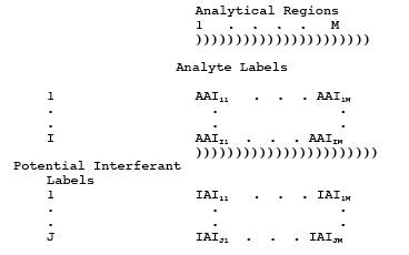
FIGURE B.2 Presentation of Known Interferant Calculations

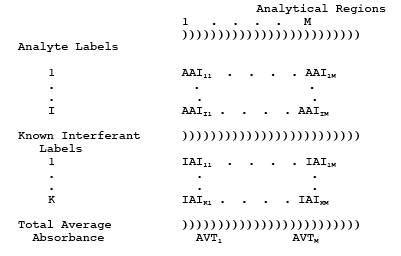
APPENDIX C TO ADDENDUM TO METHOD 320

ESTIMATING NOISE LEVELS

C.1 General

C.1.1 The root-mean-square (RMS) noise level is the standard measure of noise in this addendum. The RMS noise level of a contiguous segment of a spectrum is defined as the RMS difference (RMSD) between the absorbance values which form the segment and the mean value of that segment (see appendix A of this addendum).

C.1.2 The RMS noise value in double-beam absorbance spectra is assumed to be inversely proportional to: (a) the square root of the signal integration period of the sample single beam spectra from which it is formed, and (b) the total infrared power transmitted through the interferometer and absorption cell.

C.1.3 Practically, the assumption of C.1.2 allows the RMS noise level of a complete system to be estimated from the quantities described in sections C.1.3.1 through C.1.3.4:

C.1.3.1 RMSMAN, the noise level of the system (in absorbance units), without the absorption cell and transfer optics, under those conditions necessary to yield the specified minimum instrumental line-width, e.g., Jacquinot stop size.

C.1.3.2 tMAN, the manufacturer's signal integration time used to determine RMSMAN.

C.1.3.3 tSS, the signal integration time for the analyses.

C.1.3.4 TP, the manufacturer's estimate of the fraction of the total infrared power transmitted by the absorption cell and transfer optics from the interferometer to the detector.

C.2 Calculations

C.2.1 Obtain the values of RMSMAN, tMAN, and TP from the manufacturers of the equipment, or determine the noise level by direct measurements with the completely constructed system proposed in section 4 of this addendum.

C.2.2 Calculate the noise value of the system (RMSEST) using equation C.1.

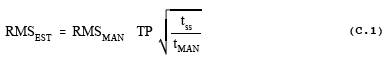
APPENDIX D TO ADDENDUM TO METHOD 320

ESTIMATING MINIMUM CONCENTRATION MEASUREMENT UNCERTAINTIES (MAU and MIU)

D.1 General

Estimate the minimum concentration measurement uncertainties for the ith analyte (MAUi) and jth interferant (MIUj) based on the spectral data in the mth analytical region by comparing the analyte band area in the analytical region (AAIim) and estimating or measuring the noise level of the system (RMSEST or RMSSm).

Note: For a single analytical region, the MAU or MIU value is the concentration of the analyte or interferant for which the band area is equal to the product of the analytical region width (in wavenumbers) and the noise level of the system (in absorbance units). If data from more than one analytical region are used in the determination of an analyte concentration, the MAU or MIU is the mean of the separate MAU or MIU values calculated for each analytical region.

D.2 Calculations

D.2.1 For each analytical region, set RMS = RMSSm if measured (appendix G of this addendum), or set RMS = RMSEST if estimated (appendix C of this addendum).

D.2.2 For each analyte associated with the analytical region, calculate MAUim using equation D.1,

D.2.3 If only the mth analytical region is used to calculate the concentration of the ith analyte, set MAUi = MAUim.

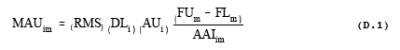
D.2.4 If more than one analytical region is used to calculate the concentration of the ith analyte, set MAUi equal to the weighted mean of the appropriate MAUim values calculated above; the weight for each term in the mean is equal to the fraction of the total wavenumber range used for the calculation represented by each analytical region. Mathematically, if the set of analytical regions employed is {m'}, then the MAU for each analytical region is given by equation D.2.

where the weight Wik is defined for each term in the sum as

D.2.5 Repeat sections D.2.1 through D.2.4 of this appendix to calculate the analogous values MIUj for the interferants j = 1 to J. Replace the value (AUi)(DLi) in equation D.1 with CPOTj/20; replace the value AAIim in equation D.1 with IAIjm.

APPENDIX E TO ADDENDUM TO METHOD 320

DETERMINING FRACTIONAL REPRODUCIBILITY UNCERTAINTIES (FRU)

E.1 General

To estimate the reproducibility of the spectroscopic results of the system, compare the CTS spectra recorded before and after preparing the reference spectra. Compare the difference between the spectra to their average band area. Perform the calculation for each analytical region on the portions of the CTS spectra associated with that analytical region.

E.2 Calculations

E.2.1 The CTS spectra {R1} consist of N spectra, denoted by S1i, i=1, N. Similarly, the CTS spectra {R2} consist of N spectra, denoted by S2i, i=1, N. Each Ski is the spectrum of a single compound, where i denotes the compound and k denotes the set {Rk} of which Ski is a member. Form the spectra S3 according to S3i = S2i-S1i for each i. Form the spectra S4 according to S4i = [S2i+S1i]/2 for each i.

E.2.2 Each analytical region m is associated with a portion of the CTS spectra S2i and S1i, for a particular i, with lower and upper wavenumber limits FFLm and FFUm, respectively.

E.2.3 For each m and the associated i, calculate the band area of S4i in the wavenumber range FFUm to FFLm. Follow the guidelines of section B.1.2 of this addendum for this band area calculation. Denote the result by BAVm.

E.2.4 For each m and the associated i, calculate the RMSD of S3i between the absorbance values and their mean in the wavenumber range FFUm to FFLm. Denote the result by SRMSm.

E.2.5 For each analytical region m, calculate FMm using equation E.1,

E.2.6 If only the mth analytical region is used to calculate the concentration of the ith analyte, set FRUi = FMm.

E.2.7 If a number pi of analytical regions are used to calculate the concentration of the ith analyte, set FRUi equal to the weighted mean of the appropriate FMm values calculated according to section E.2.5. Mathematically, if the set of analytical regions employed is {m'}, then FRUi is given by equation E.2,

where the Wik are calculated as described in appendix D of this addendum.

APPENDIX F OF ADDENDUM TO METHOD 320

DETERMINING FRACTIONAL CALIBRATION UNCERTAINTIES (FCU)

F.1 General

F.1.1 The concentrations yielded by the computerized analytical program applied to each single-compound reference spectrum are defined as the indicated standard concentrations (ISC's). The ISC values for a single compound spectrum should ideally equal the accepted standard concentration (ASC) for one analyte or interferant, and should ideally be zero for all other compounds. Variations from these results are caused by errors in the ASC values, variations from the Beer's law (or modified Beer's law) model used to determine the concentrations, and noise in the spectra. When the first two effects dominate, the systematic nature of the errors is often apparent and the analyst shall take steps to correct them.

F.1.2 When the calibration error appears nonsystematic, apply the procedures of sections F.2.1 through F.2.3 of this appendix to estimate the fractional calibration uncertainty (FCU) for each compound. The FCU is defined as the mean fractional error between the ASC and the ISC for all reference spectra with non-zero ASC for that compound. The FCU for each compound shall be less than the required fractional uncertainty specified in section 4.1 of this addendum.

F.1.3 The computerized analytical programs shall also be required to yield acceptably low concentrations for compounds with ISC = 0 when applied to the reference spectra. The ISC of each reference spectrum for each analyte or interferant shall not exceed that compound's minimum measurement uncertainty (MAU or MIU).

F.2 Calculations

F.2.1 Apply each analytical program to each reference spectrum. Prepare a similar table to that in Figure F.1 to present the ISC and ASC values for each analyte and interferant in each reference spectrum. Maintain the order of reference file names and compounds employed in preparing Figure F.1.

F.2.2 For all reference spectra in Figure F.1, verify that the absolute values of the ISC's are less than the compound's MAU (for analytes) or MIU (for interferants).

F.2.3 For each analyte reference spectrum, calculate the quantity (ASC-ISC)/ASC. For each analyte, calculate the mean of these values (the FCUi for the ith analyte) over all reference spectra. Prepare a similar table to that in Figure F.2 to present the FCUi and analytical uncertainty limit (AUi) for each analyte.

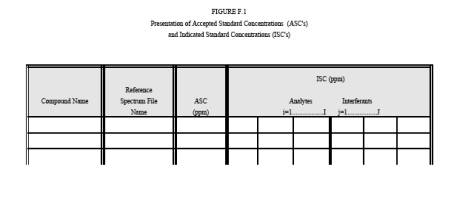
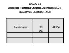
APPENDIX G TO ADDENDUM TO METHOD 320

MEASURING NOISE LEVELS

G.1 General

The root-mean-square (RMS) noise level is the standard measure of noise. The RMS noise level of a contiguous segment of a spectrum is the RMSD between the absorbance values that form the segment and the mean value of the segment (see appendix A of this addendum).

G.2 Calculations

G.2.1 Evacuate the absorption cell or fill it with UPC grade nitrogen at approximately one atmosphere total pressure.

G.2.2 Record two single beam spectra of signal integration period tSS.

G.2.3 Form the double beam absorption spectrum from these two single beam spectra, and calculate the noise level RMSSm in the M analytical regions.

APPENDIX H OF ADDENDUM TO METHOD 320

DETERMINING SAMPLE ABSORPTION PATHLENGTH (LS) AND FRACTIONAL ANALYTICAL UNCERTAINTY (FAU)

H.1 General

Reference spectra recorded at absorption pathlength (LR), gas pressure (PR), and gas absolute temperature (TR) may be used to determine analyte concentrations in samples whose spectra are recorded at conditions different from that of the reference spectra, i.e., at absorption pathlength (LS), absolute temperature (TS), and pressure (PS). This appendix describes the calculations for estimating the fractional uncertainty (FAU) of this practice. It also describes the calculations for determining the sample absorption pathlength from comparison of CTS spectra, and for preparing spectra for further instrumental and procedural checks.

H.1.1 Before sampling, determine the sample absorption pathlength using least squares analysis. Determine the ratio LS/LR by comparing the spectral sets {R1} and {R3}, which are recorded using the same CTS at LS and LR, and TS and TR, but both at PR.

H.1.2 Determine the fractional analysis uncertainty (FAU) for each analyte by comparing a scaled CTS spectral set, recorded at LS, TS, and PS, to the CTS reference spectra of the same gas, recorded at LR, TR, and PR. Perform the quantitative comparison after recording the sample spectra, based on band areas of the spectra in the CTS absorbance band associated with each analyte.

H.2 Calculations

H.2.1 Absorption Pathlength Determination. Perform and document separate linear baseline corrections to each analytical region in the spectral sets {R1} and {R3}. Form a one-dimensional array AR containing the absorbance values from all segments of {R1} that are associated with the analytical regions; the members of the array are ARi, i = 1, n. Form a similar one-dimensional array AS from the absorbance values in the spectral set {R3}; the members of the array are ASi, i = 1, n. Based on the model AS = rAR + E, determine the least-squares estimate of r', the value of r which minimizes the square error E2. Calculate the sample absorption pathlength, LS, using equation H.1,

H.2.2 Fractional Analysis Uncertainty. Perform and document separate linear baseline corrections to each analytical region in the spectral sets {R1} and {R4}. Form the arrays AS and AR as described in section H.2.1 of this appendix, using values from {R1} to form AR, and values from {R4} to form AS. Calculate NRMSE and IAAV using equations H.2 and H.3,

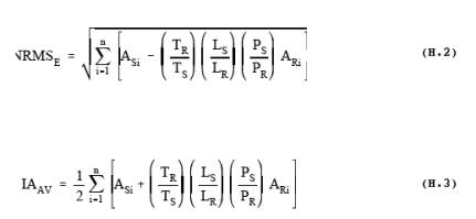
The fractional analytical uncertainty, FAU, is given by equation H.4,

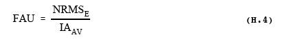
APPENDIX I TO ADDENDUM TO METHOD 320

DETERMINING FRACTIONAL MODEL UNCERTAINTIES (FMU)

I.1 General

To prepare analytical programs for FTIR analyses, the sample constituents must first be assumed. The calculations in this appendix, based upon a simulation of the sample spectrum, shall be used to verify the appropriateness of these assumptions. The simulated spectra consist of the sum of single compound reference spectra scaled to represent their contributions to the sample absorbance spectrum; scaling factors are based on the indicated standard concentrations (ISC) and measured (sample) analyte and interferant concentrations, the sample and reference absorption pathlengths, and the sample and reference gas pressures. No band-shape correction for differences in the temperature of the sample and reference spectra gases is made; such errors are included in the FMU estimate. The actual and simulated sample spectra are quantitatively compared to determine the fractional model uncertainty; this comparison uses the reference spectra band areas and residuals in the difference spectrum formed from the actual and simulated sample spectra.

I.2 Calculations

I.2.1 For each analyte (with scaled concentration RSAi), select a reference spectrum SAi with indicated standard concentration ISCi. Calculate the scaling factors, RAi, using equation I.1,

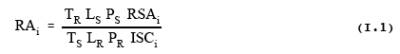
Form the spectra SACi by scaling each SAi by the factor RAi.

I.2.2 For each interferant, select a reference spectrum SIk with indicated standard concentration ISCk. Calculate the scaling factors, RIk, using equation I.2,

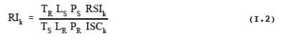
Form the spectra SICk by scaling each SIk by the factor RIk.

I.2.3 For each analytical region, determine by visual inspection which of the spectra SACi and SICk exhibit absorbance bands within the analytical region. Subtract each spectrum SACi and SICk exhibiting absorbance from the sample spectrum SS to form the spectrum SUBS. To save analysis time and to avoid the introduction of unwanted noise into the subtracted spectrum, it is recommended that the calculation be made (1) only for those spectral data points within the analytical regions, and (2) for each analytical region separately using the original spectrum SS.

I.2.4 For each analytical region m, calculate the RMSD of SUBS between the absorbance values and their mean in the region FFUm to FFLm. Denote the result by RMSSm.

I.2.5 For each analyte i, calculate FMm, using equation I.3,

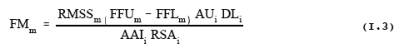
for each analytical region associated with the analyte.

I.2.6 If only the mth analytical region is used to calculate the concentration of the ith analyte, set FMUi=FMm.

I.2.7 If a number of analytical regions are used to calculate the concentration of the ith analyte, set FMi equal to the weighted mean of the appropriate FMm values calculated using equation I-3. Mathematically, if the set of analytical regions employed is {m'}, then the fractional model uncertainty, FMU, is given by equation I.4,

where Wik is calculated as described in appendix D of this addendum.

APPENDIX J OF ADDENDUM TO METHOD 320

DETERMINING OVERALL CONCENTRATION UNCERTAINTIES (OCU)

The calculations in this addendum estimate the measurement uncertainties for various FTIR measurements. The lowest possible overall concentration uncertainty (OCU) for an analyte is its MAU value, which is an estimate of the absolute concentration uncertainty when spectral noise dominates the measurement error. However, if the product of the largest fractional concentration uncertainty (FRU, FCU, FAU, or FMU) and the measured concentration of an analyte exceeds the MAU for the analyte, then the OCU is this product. In mathematical terms, set OFUi = MAX{FRUi, FCUi, FAUi, FMUi} and OCUi = MAX{RSAi*OFUi, MAUi}.

Figure 2. FTIR Sampling/Spiking System.