This method, as specified in the applicable subpart, is to be used whenever a source owner or operator (hereafter referred to as an "analyst") proposes a test method to meet a U.S. Environmental Protection Agency (EPA) requirement in the absence of a validated method. This Method includes procedures for determining and documenting the quality, i.e., systematic error (bias) and random error (precision), of the measured concentrations from an effected source. This method is applicable to various waste media (i.e., exhaust gas, wastewater, sludge, etc.).

1.1.1 If EPA currently recognizes an appropriate test method or considers the analyst's test method to be satisfactory for a particular source, the Administrator may waive the use of this protocol or may specify a less rigorous validation procedure. A list of validated methods may be obtained by contacting the Emission Measurement Technical Information Center (EMTIC), Mail Drop 19, U.S. Environmental Protection Agency, Research Triangle Park, NC 27711, 919/541-0200. Procedures for obtaining a waiver are in Section 12.0.

1.1.2 This method includes optional procedures that may be used to expand the applicability of the proposed method. Section 7.0 involves ruggedness testing (Laboratory Evaluation), which demonstrates the sensitivity of the method to various parameters. Section 8.0 involves a procedure for including sample stability in bias and precision for assessing sample recovery and analysis times; Section 9.0 involves a procedure for the determination of the practical limit of quantitation for determining the lower limit of the method. These optional procedures are required for the waiver consideration outlined in Section 12.0.

1.2 Principle.

The purpose of these procedures is to determine bias and precision of a test method at the level of the applicable standard. The procedures involve (a) introducing known concentrations of an analyte or comparing the test method against a validated test method to determine the method's bias and (b) collecting multiple or collocated simultaneous samples to determine the method's precision.

1.2.1 Bias.

Bias is established by comparing the method's results against a reference value and may be eliminated by employing a correction factor established from the data obtained during the validation test. An offset bias may be handled accordingly. Methods that have bias correction factors outside 0.7 to 1.3 are unacceptable. Validated method to proposed method comparisons, Section 6.2, requires a more restrictive test of central tendency and a lower correction factor allowance of 0.90 to 1.10.

1.2.2 Precision.

At the minimum, paired sampling systems shall be used to establish precision. The precision of the method at the level of the standard shall not be greater than 50 percent relative standard deviation. For a validated method to proposed method equivalency comparisons, Section 6.2, the analyst must demonstrate that the precision of the proposed test method is as precise as the validated method for acceptance.

2. DEFINITIONS

2.1 Negative bias. Bias Resulting when the measured result is less than the "true" value.

2.2 Paired sampling system. A sampling system capable of obtaining two replicate samples that were collected as closely as possible in sampling time and sampling location.

2.3 Positive bias. Bias resulting when the measured result is greater than the "true" value.

2.4 Proposed method. The sampling and analytical methodology selected for field validation using the method described herein.

2.5 Quadruplet sampling system. A sampling system capable of obtaining four replicate samples that were collected as closely as possible in sampling time and sampling location.

2.6 Surrogate compound. A compound that serves as a model for the types of compounds being analyzed (i.e., similar chemical structure, properties, behavior). The model can be distinguished by the method from the compounds being analyzed.

3. REFERENCE MATERIAL

The reference materials shall be obtained or prepared at the level of the standard. Additional runs with higher and lower reference material concentrations may be made to expand the applicable range of the method, in accordance with the ruggedness test procedures.

3.1 Exhaust Gas Tests.

The analyst shall obtain a known concentration of the reference material (i.e., analyte of concern) from an independent source such as a specialty gas manufacturer, specialty chemical company, or commercial laboratory. A list of vendors may be obtained from EMTIC (see Section 1.1.1). The analyst should obtain the manufacturer's stability data of the analyte concentration and recommendations for recertification.

3.2 Other Waste Media Tests.

The analyst shall obtain pure liquid components of the reference materials (i.e., analytes of concern) from an independent manufacturer and dilute them in the same type matrix as the source waste. The pure reference materials shall be certified by the manufacturer as to purity and shelf life. The accuracy of all diluted reference material concentrations shall be verified by comparing their response to independently-prepared materials (independently prepared in this case means prepared from pure components by a different analyst).

3.3 Surrogate Reference Materials.

The analyst may use surrogate compounds, e.g., for highly toxic or reactive organic compounds, provided the analyst can demonstrate to the Administrator's satisfaction that the surrogate compound behaves as the analyte. A surrogate may be an isotope or one that contains a unique element (e.g., chlorine) that is not present in the source or a derivative of the toxic or reactive compound, if the derivative formation is part of the method's procedure. Laboratory experiments or literature data may be used to show behavioral acceptability.

3.4 Isotopically Labeled Materials.

Isotope mixtures may contain the isotope and the natural analyte. For best results, the isotope labeled analyte concentration should be more than five times the natural concentration of the analyte.

4. EPA PERFORMANCE AUDIT MATERIAL

4.1 To assess the method bias independently, the analyst shall use (in addition to the reference material) an EPA performance audit material, if it is available. The analyst may contact EMTIC (see Section 1.1.1) to receive a list of currently available EPA audit materials. If the analyte is listed, the analyst should request the audit material at least 30 days before the validation test. If an EPA audit material is not available, request documentation from the validation report reviewing authority that the audit material is currently not available from EPA. Include this documentation with the field validation report.

4.2 The analyst shall sample and analyze the performance audit sample three times according to the instructions provided with the audit sample. The analyst shall submit the three results with the field validation report. Although no acceptance criteria are set for these performance audit results, the analyst and reviewing authority may use them to assess the relative error of sample recovery, sample preparation, and analytical procedures and then consider the relative error in evaluating the measured emissions.

5. PROCEDURE FOR DETERMINATION OF BIAS AND PRECISION IN THE FIELD

The analyst shall select one of the sampling approaches below to determine the bias and precision of the data. After analyzing the samples, the analyst shall calculate the bias and precision according to the procedure described in Section 6.0. When sampling a stationary source, follow the probe placement procedures in Section 5.4.

5.1 Isotopic Spiking.

This approach shall be used only for methods that require mass spectrometry (MS) analysis. Bias and precision are calculated by procedures described in Section 6.1.

5.1.1 Number of Samples and Sampling Runs. Collect a total of 12 replicate samples by either obtaining six sets of paired samples or three sets of quadruplet samples.

5.1.2 Spiking Procedure. Spike all 12 samples with the reference material at the level of the standard. Follow the appropriate spiking procedures listed below for the applicable waste medium.

5.1.2.1 Exhaust Gas Testing. The spike shall be introduced as close to the tip of the sampling probe as possible.

5.1.2.1.1 Gaseous Reference Material with Sorbent or Impinger Sampling Trains. Sample the reference material (in the laboratory or in the field) at a concentration which is close to the allowable concentration standard for the time required by the method, and then sample the gas stream for an equal amount of time. The time for sampling both the reference material and gas stream should be equal; however, the time should be adjusted to avoid sorbent breakthrough.

5.1.2.1.2 Gaseous Reference Material with Sample Container (Bag or Canister). Spike the sample containers after completion of each test run with an amount equal to the allowable concentration standard of the emission point. The final concentration of the reference material shall approximate the level of the emission concentration in the stack. The volume amount of reference material shall be less than 10 percent of the sample volume.

5.1.2.1.3 Liquid and Solid Reference Material with Sorbent or Impinger Trains. Spike the trains with an amount equal to the allowable concentration standard before sampling the stack gas. The spiking should be done in the field; however, it may be done in the laboratory.

5.1.2.1.4 Liquid and Solid Reference Material with Sample Container (Bag or Canister). Spike the containers at the completion of each test run with an amount equal to the level of the emission standard.

5.1.2.2 Other Waste Media. Spike the 12 replicate samples with the reference material either before or directly after sampling in the field.

5.2 Comparison Against a Validated Test Method.

Bias and precision are calculated using the procedures described in Section 6.2. This approach shall be used when a validated method is available and an alternative method is being proposed.

5.2.1 Number of Samples and Sampling Runs. Collect nine sets of replicate samples using a paired sampling system (a total of 18 samples) or four sets of replicate samples using a quadruplet sampling system (a total of 16 samples). In each sample set, the validated test method shall be used to collect and analyze half of the samples.

5.2.2 Performance Audit Exception. Conduct the performance audit as required in Section 4.0 for the validated test method. Conducting a performance audit on the test method being evaluated is recommended.

5.3 Analyte Spiking.

This approach shall be used when Sections 5.1 and 5.2 are not applicable. Bias and precision are calculated using the procedures described in Section 6.3.

5.3.1 Number of Samples and Sampling Runs. Collect a total of 24 samples using the quadruplet sampling system (a total of 6 sets of replicate samples).

5.3.2 In each quadruplet set, spike half of the samples (two out of the four) with the reference material according to the applicable procedure in Section 5.1.2.1 or 5.1.2.2.

5.4 Probe Placement and Arrangement For Stationary Source Stack or Duct Sampling.

The probes shall be placed in the same horizontal plane. For paired sample probes the arrangement should be that the probe tip is 2.5 cm from the outside edge of the other with a pitot tube on the outside of each probe. Other paired arrangements for the pitot tube may be acceptable. For quadruplet sampling probes, the tips should be in a 6.0 cm x 6.0 cm square area measured from the center line of the opening of the probe tip with a single pitot tube in the center or two pitot tubes with their location on either side of the probe tip configuration. An alternative arrangement should be proposed when ever the cross-sectional area of the probe tip configuration is approximately 5 percent of the stack or duct cross-sectional area.

6. CALCULATIONS

Data resulting from the procedures specified in Section 5.0 shall be treated as follows to determine bias, correction factors, relative standard deviations, precision, and data acceptance.

6.1 Isotopic Spiking.

Analyze the data for isotopic spiking tests as outlined in Sections 6.1.1 through 6.1.6.

6.1.1 Calculate the numerical value of the bias using the results from the analysis of the isotopically spiked field samples and the calculated value of ENDFIELD the isotopically labeled spike:

where:

B = Bias at the spike level.

Sm = Mean of the measured values of the isotopically spiked samples.

CS = Calculated value of the isotopically labeled spike.

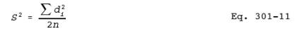
6.1.2 Calculate the standard deviation of the Si values as follows:

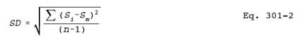
where:

Si = Measured value of the isotopically labeled analyte in the ith field sample,

n = Number of isotopically spiked samples, 12.

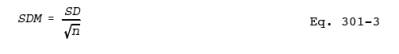
6.1.3 Calculate the standard deviation of the mean (SDM) as follows:

6.1.4 Test the bias for statistical significance by calculating the t-statistic,

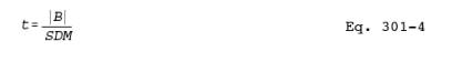
and compare it with the critical value of the two-sided t-distribution at the 95-percent confidence level and n-1 degrees of freedom. This critical value is 2.201 for the eleven degrees of freedom when the procedure specified in Section 5.1.2 is followed. If the calculated t-value is greater than the critical value the bias is statistically significant and the analyst should proceed to evaluate the correction factor.

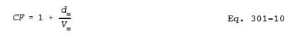
6.1.5 Calculation of a Correction Factor. If the t-test does not show that the bias is statistically significant, use all analytical results without correction and proceed to the precision evaluation. If the method's bias is statistically significant, calculate the correction factor, CF, using the following equation:

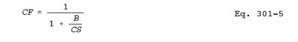
If the CF is outside the range of 0.70 to 1.30, the data and method are considered unacceptable. For correction factors within the range, multiply all analytical results by the CF to obtain the final values.

6.1.6 Calculation of the Relative Standard Deviation (Precision). Calculate the relative standard deviation as follows:

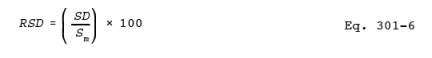
where Sm is the measured mean of the isotopically labeled spiked samples.

6.2 Comparison with Validated Method.

Analyze the data for comparison with a validated method as outlined in Sections 6.2.1 or 6.2.2, as appropriate. Conduct these procedures in order to determine if a proposed method produces results equivalent to a validated method. Make all necessary bias corrections for the validated method, as appropriate. If the proposed method fails either test, the method results are unacceptable, and conclude that the proposed method is not as precise or accurate as the validated method. For highly variable sources, additional precision checks may be necessary. The analyst should consult with the Administrator if a highly variable source is suspected.

6.2.1 Paired Sampling Systems.

6.2.1.1 Precision. Determine the acceptance of the proposed method's variance with respect to the variability of the validated method results. If a significant difference is determined, the proposed method and the results are rejected. Proposed methods demonstrating F-values equal to or less than the critical value have acceptable precision.

6.2.1.2 Calculate the variance of the proposed method, Sp 2 and the variance of the validated method, Sv 2, using the following equation:

where:

SDv = Standard deviation provided with the validated method,

SDp = Standard deviation of the proposed method calculated using Equation 301-9a.

6.2.1.3 The F-test. Determine if the variance of the proposed method is significantly different from that of the validated method by calculating the F-value using the following equation:

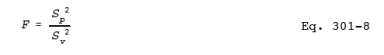
Compare the experimental F value with the critical value of F. The critical value is 1.0 when the procedure specified in section 5.2.1 for paired trains is followed. If the calculated F is greater than the critical value, the difference in precision is significant and the data and proposed method are unacceptable.

6.2.1.4 Bias Analysis. Test the bias for statistical significance by calculating the t-statistic and determine if the mean of the differences between the proposed method and the validated method is significant at the 80-percent confidence level. This procedure requires the standard deviation of the validated method, SDv, to be known. Employ the value furnished with the method. If the standard deviation of the validated method is not available, the paired replicate sampling procedure may not be used. 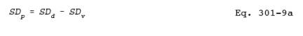Determine the mean of the paired sample differences, dm, and the standard deviation, SDd, of the differences, di's, using Equation 301-2 where: di replaces Si, dm replaces Sm. Calculate the standard deviation of the proposed method, SDp, as follows:

(If SDv > SDd, let SD = SDd/1.414). Calculate the value of the t-statistic using the following

equation:

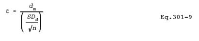
where n is the total number of paired samples. For the procedure in Section 5.2.1, n equals nine. Compare the calculated t-statistic with the corresponding value from the table of the t-statistic. When nine runs are conducted, as specified in Section 5.2.1, the critical value of the t-statistic is 1.397 for eight degrees of freedom. If the calculated t-value is greater than the critical value the bias is statistically significant and the analyst should proceed to evaluate the correction factor.

6.2.1.5 Calculation of a Correction Factor. If the statistical test cited above does not show a significant bias with respect to the reference method, assume that the proposed method is unbiased and use all analytical results without correction. If the method's bias is statistically significant, calculate the correction factor, CF, as follows:

where Vm is the mean of the validated method's values. Multiply all analytical results by CF to obtain the final values. The method results, and the method, are unacceptable if the correction factor is outside the range of 0.9 to 1.10.

6.2.2 Quadruplet Replicate Sampling Systems.

6.2.2.1 Precision. Determine the acceptance of the proposed method's variance with respect to the variability of the validated method results. If a significant difference is determined the proposed method and the results are rejected.

6.2.2.2 Calculate the variance of the proposed method, Sp 2 using the following equation:

where the di's are the differences between the validated method values and the proposed method values.

6.2.2.3 The F-test. Determine if the variance of the proposed method is more variable than that of the validated method by calculating the F-value using Equation 301-8. Compare the experimental F value with the critical value of F. The critical value is 1.0 when the procedure specified in section 5.2.2 for quadruplet trains is followed. The calculated F should be less than or equal to the critical value. If the difference in precision is significant the results and the proposed method are unacceptable.

6.2.2.4 Bias Analysis. Test the bias for statistical significance at the 80 percent confidence level by calculating the t-statistic. Determine the bias (mean of the differences between the proposed method and the validated method, dm) and the standard deviation, SDd, of the differences. Calculate the standard deviation of the differences, SDd, using Equation 301-2 and substituting di for Si. The following equation is used to calculate di:

and: V1i = First measured value of the validated method in the ith test sample.

P1i = First measured value of the proposed method in the ith test sample.

Calculate the t-statistic using Equation 301-9 where n is the total number of test sample differences (di). For the procedure in Section 5.2.2, n equals four. Compare the calculated t-statistic with the corresponding value from the table of the t-statistic and determine if the mean is significant at the 80-percent confidence level. When four runs are conducted, as specified in Section 5.2.2, the critical value of the t-statistic is 1.638 for three degrees of freedom. If the calculated t-value is greater than the critical value the bias is statistically significant and the analyst should proceed to evaluate the correction factor.

6.2.2.5 Correction Factor Calculation. If the method's bias is statistically significant, calculate the correction factor, CF, using Equation 301-10. Multiply all analytical results by CF to obtain the final values. The method results, and the method, are unacceptable if the correction factor is outside the range of 0.9 to 1.10.

6.3 Analyte Spiking.

Analyze the data for analyte spike testing as outlined in Sections 6.3.1 through 6.3.3.

6.3.1 Precision.

6.3.1.1 Spiked Samples. Calculate the difference, di, between the pairs of the spiked proposed method measurements for each replicate sample set. Determine the standard deviation (SDs) of the spiked values using the following equation:

where: n = Number of paired samples.

Calculate the relative standard deviation of the proposed spiked method using Equation 301-6 where Sm is the measured mean of the analyte spiked samples. The proposed method is unacceptable if the RSD is greater than 50 percent.

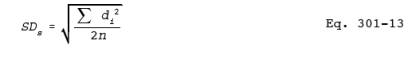
6.3.1.2 Unspiked Samples. Calculate the standard deviation of the unspiked values using Equation 301-13 and the relative standard deviation of the proposed unspiked method using Equation 301-6 where Sm is the measured mean of the unspiked samples. The RSD must be less than or equal to 50 percent.

6.3.2 Bias.

Calculate the numerical value of the bias using the results from the analysis of the spiked field samples, the unspiked field samples, and the calculated value of the spike:

where:

B = Bias at the spike level.

Sm = Mean of the spiked samples.

Mm = Mean of the unspiked samples.

CS = Calculated value of the spiked level.

6.3.2.1 Calculate the standard deviation of the mean using the following equation where SDs and SDu are the standard deviations of the spiked and unspiked sample values respectively as calculated using Equation 301-13.

6.3.2.2 Test the bias for statistical significance by calculating the t- statistic using Equation 301-4 and comparing it with the critical value of the two-sided t-distribution at the 95-percent confidence level and n-1 degrees of freedom. This critical value is 2.201 for the eleven degrees of freedom.

6.3.3 Calculation of a Correction Factor.

If the t-test shows that the bias is not statistically significant, use all analytical results without correction. If the method's bias is statistically significant, calculate the correction factor using Equation 301-5. Multiply all analytical results by CF to obtain the final values.

7. RUGGEDNESS TESTING (OPTIONAL)

7.1 Laboratory Evaluation.

7.1.1 Ruggedness testing is a useful and cost-effective laboratory study to determine the sensitivity of a method to certain parameters such as sample collection rate, interferant concentration, collecting medium temperature, or sample recovery temperature. This Section generally discusses the principle of the ruggedness test. A more detailed description is presented in citation 10 of Section 13.0.

7.1.2 In a ruggedness test, several variables are changed simultaneously rather than one variable at a time. This reduces the number of experiments required to evaluate the effect of a variable. For example, the effect of seven variables can be determined in eight experiments rather than 128 (W.J. Youden, Statistical Manual of the Association of Official Analytical Chemists, Association of Official Analytical Chemists, Washington, DC, 1975, pp. 33-36).

7.1.3 Data from ruggedness tests are helpful in extending the applicability of a test method to different source concentrations or source categories.

8. PROCEDURE FOR INCLUDING SAMPLE STABILITY IN BIAS AND PRECISION EVALUATIONS

8.1 Sample Stability.

8.1.1 The test method being evaluated must include procedures for sample storage and the time within which the collected samples shall be analyzed.

8.1.2 This Section identifies the procedures for including the effect of storage time in bias and precision evaluations. The evaluation may be deleted if the test method specifies a time

for sample storage.

8.2 Stability Test Design.

The following procedures shall be conducted to identify the effect of storage times on analyte samples. Store the samples according to the procedure specified in the test method. When using the analyte spiking procedures (Section 5.3), the study should include equal numbers of spiked and unspiked samples.

8.2.1 Stack Emission Testing.

8.2.1.1 For sample container (bag or canister) and impinger sampling systems, Sections 5.1 and 5.3, analyze six of the samples at the minimum storage time. Then analyze the same six samples at the maximum storage time.

8.2.1.2 For sorbent and impinger sampling systems, Sections 5.1 and 5.3, that require extraction or digestion, extract or digest six of the samples at the minimum storage time and extract or digest six other samples at the maximum storage time. Analyze an aliquot of the first six extracts (digestates) at both the minimum and maximum storage times. This will provide some freedom to analyze extract storage impacts.

8.2.1.3 For sorbent sampling systems, Sections 5.1 and 5.3, that require thermal desorption, analyze six samples at the minimum storage time. Analyze another set of six samples at the maximum storage time.

8.2.1.4 For systems set up in accordance with Section 5.2, the number of samples analyzed at the minimum and maximum storage times shall be half those collected (8 or 9). The procedures for samples requiring extraction or digestion should parallel those

in Section 8.2.1.

8.2.2 Other Waste Media Testing.

Analyze half of the replicate samples at the minimum storage time and the other half at the maximum storage time in order to identify the effect of storage times on analyte samples.

9. PROCEDURE FOR DETERMINATION OF PRACTICAL LIMIT OF QUANTITATION (OPTIONAL)

9.1 Practical Limit of Quantitation.

9.1.1 The practical limit of quantitation (PLQ) is the lowest level above which quantitative results may be obtained with an acceptable degree of confidence. For this protocol, the PLQ is defined as 10 times the standard deviation, so, at the blank level. This PLQ corresponds to an uncertainty of ±30 percent at the 99-percent confidence level.

9.1.2 The PLQ will be used to establish the lower limit of the test method.

9.2 Procedure I for Estimating so.

This procedure is acceptable if the estimated PLQ is no more than twice the calculated PLQ. If the PLQ is greater than twice the calculated PLQ use Procedure II.

9.2.1 Estimate the PLQ and prepare a test standard at this level. The test standard could consist of a dilution of the reference material described in Section 3.0.

9.2.2 Using the normal sampling and analytical procedures for the method, sample and analyze this standard at least seven times in the laboratory.

9.2.3 Calculate the standard deviation, so, of the measured values.

9.2.4 Calculate the PLQ as 10 times so.

9.3 Procedure II for Estimating so.

This procedure is to be used if the estimated PLQ is more than twice the calculated PLQ.

9.3.1 Prepare two additional standards at concentration levels lower than the standard used in Procedure I.

9.3.2 Sample and analyze each of these standards at least seven times.

9.3.3 Calculate the standard deviation for each concentration level.

9.3.4 Plot the standard deviations of the three test standards as a function of the standard concentrations.

9.3.5 Draw a best-fit straight line through the data points and extrapolate to zero concentration. The standard deviation at zero concentration is so.

9.3.6 Calculate the PLQ as 10 times so.

10.0 FIELD VALIDATION REPORT REQUIREMENTS

The field validation report shall include a discussion of the regulatory objectives for the testing which describe the reasons for the test, applicable emission limits, and a description of the source. In addition, validation results shall include:

10.1 Summary of the results and calculations shown in Section 6.0.

10.2 Reference material certification and value(s).

10.3 Performance audit results or letter from the reviewing authority stating the audit material is currently not available.

10.4 Laboratory demonstration of the quality of the spiking system.

10.5 Discussion of laboratory evaluations.

10.6 Discussion of field sampling.

10.7 Discussion of sample preparations and analysis.

10.8 Storage times of samples (and extracts, if applicable).

10.9 Reasons for eliminating any results.

11. FOLLOWUP TESTING

The correction factor calculated in Section 6.0 shall be used to adjust the sample concentrations in all followup tests conducted at the same source. These tests shall consist of at least three replicate samples, and the average shall be used to determine the pollutant concentration. The number of samples to be collected and analyzed shall be as follows, depending on the validated method precision level:

11.1 Validated relative standard deviation (RSD) < ±15 Percent. Three replicate samples.

11.2 Validated RSD < ±30 Percent. Six replicate samples.

11.3 Validated RSD < ±50 Percent. Nine replicate samples.

11.4 Equivalent method. Three replicate samples.

12. PROCEDURE FOR OBTAINING A WAIVER

12.1 Waivers.

These procedures may be waived or a less rigorous protocol may be granted for site-specific applications. The following are three example situations for which a waiver may be considered.

12.1.1 "Similar" Sources.

If the test method has been validated previously at a "similar" source, the procedures may be waived provided the requester can demonstrate to the satisfaction of the Administrator that the sources are "similar." The methods's applicability to the "similar" source may be demonstrated by conducting a ruggedness test as described in Section 6.0.

12.1.2 "Documented " Methods.

In some cases, bias and precision may have been documented through laboratory tests or protocols different from this method. If the analyst can demonstrate to the satisfaction of the Administrator that the bias and precision apply to a particular application, the Administrator may waive these procedures or parts of the procedures.

12.1.3 "Conditional" Test Methods.

When the method has been demonstrated to be valid at several sources, the analyst may seek a "conditional" method designation from the Administrator. "Conditional" method status provides an automatic waiver from the procedures provided the test method is used within the stated applicability.

12.2 Application for Waiver.

In general, the requester shall provide a thorough description of the test method, the intended application, and results of any validation or other supporting documents. Because of the many potential situations in which the Administrator may grant a waiver, it is neither possible nor desirable to prescribe the exact criteria for a waiver. At a minimum, the requester is responsible for providing the following.

12.2.1 A clearly written test method, preferably in the format of 40 CFR 60, Appendix A Test Methods. The method must include an applicability statement, concentration range, precision, bias (accuracy), and time in which samples must be analyzed.

12.2.2.2 Summaries (see Section 10.0) of previous validation tests or other supporting documents. If a different procedure from that described in this method was used, the requester shall provide appropriate documents substantiating (to the satisfaction of the Administrator) the bias and precision values.

12.2.2.3 Results of testing conducted with respect to Sections 7.0, 8.0, and 9.0.

12.2.3 Discussion of the applicability statement and arguments for approval of the waiver. This discussion should address as applicable the following: Applicable regulation, emission standards, effluent characteristics, and process operations.

12.3 Requests for Waiver.

Each request shall be in writing and signed by the analyst. Submit requests to the Director, OAQPS, Technical Support Division, U.S. Environmental Protection Agency, Research Triangle Park, NC 27711.

13. BIBLIOGRAPHY

1. Albritton, J.R., G.B. Howe, S.B. Tompkins, R.K.M. Jayanty, and C.E. Decker. 1989. Stability of Parts-Per-Million Organic Cylinder Gases and Results of Source Test Analysis Audits, Status Report No. 11. Environmental Protection Agency Contract 68-02- 4125. Research Triangle Institute, Research Triangle Park, NC. September.

2. DeWees, W.G., P.M. Grohse, K.K. Luk, and F.E. Butler. 1989. Laboratory and Field Evaluation of a Methodology for Speciating Nickel Emissions from Stationary Sources. EPA Contract 68-02-4442. Prepared for Atmospheric Research and Environmental Assessment Laboratory, Office of Research and Development, U.S. Environmental Protection Agency, Research Triangle Park, NC 27711. January. 23

3. Keith, L.H., W. Crummer, J. Deegan Jr., R.A. Libby, J.K. Taylor, and G. Wentler. 1983. Principles of Environmental Analysis. American Chemical Society, Washington, DC.

4. Maxwell, E.A. 1974. Estimating variances from one or two measurements on each sample. Amer. Statistician 28:96-97.

5. Midgett, M.R. 1977. How EPA Validates NSPS Methodology. Environ. Sci. & Technol. 11(7):655-659.

6. Mitchell, W.J., and M.R. Midgett. 1976. Means to evaluate performance of stationary source test methods. Environ. Sci. & Technol. 10:85-88.

7. Plackett, R.L., and J.P. Burman. 1946. The design of optimum multifactorial experiments. Biometrika, 33:305.

8. Taylor, J.K. 1987. Quality Assurance of Chemical Measurements. Lewis Publishers, Inc., pp. 79-81.

9. U.S. Environmental Protection Agency. 1978. Quality Assurance Handbook for Air Pollution Measurement Systems: Volume III. Stationary Source Specific Methods. Publication No. EPA-600/4-77-027b. Office of Research and Development Publications, 26 West St. Clair St., Cincinnati, OH 45268.

10. U.S. Environmental Protection Agency. 1981. A Procedure for Establishing Traceability of Gas Mixtures to Certain National Bureau of Standards Standard Reference Materials. Publication No. EPA-600/7-81-010. Available from the U.S. EPA, Quality Assurance Division (MD-77), Research Triangle Park, NC 27711.

11. U.S. Environmental Protection Agency. 1991. Protocol for The Field Validation of Emission Concentrations From Stationary Sources. Publication No. 450/4-90-015. Available from the U.S. EPA, Emission Measurement Technical Information Center, Technical Support Division (MD-14), Research Triangle Park, NC 27711.

12. Youdon, W.J. Statistical techniques for collaborative tests. In: Statistical Manual of the Association of Official Analytical Chemists, Association of Official Analytical Chemists,

Washington, DC, 1975, pp. 33-36.