This method applies to the in-stack measurement of particulate matter (PM) emissions equal to or less than an aerodynamic diameter of nominally 10 µm (PM10) from stationary sources. The EPA recognizes that condensible emissions not collected by an in-stack method are also PM10, and that emissions that contribute to ambient PM10 levels are the sum of condensible emissions and emissions measured by an in-stack PM10 method, such as this method or Method 201. Therefore, for establishing source contributions to ambient levels of PM10, such as for emission inventory purposes, EPA suggests that source PM10 measurement include both in-stack PM10 and condensible emissions. Condensible emissions may be measured by an impinger analysis in combination with this method.

1.2 Principle.

A gas sample is extracted at a constant flow rate through an in-stack sizing device, which separates PM greater than PM10. Variations from isokinetic sampling conditions are maintained within well-defined limits. The particulate mass is determined gravimetrically after removal of uncombined water.

2. Apparatus

NOTE: Methods cited in this method are part of 40 CFR Part 60, Appendix A.

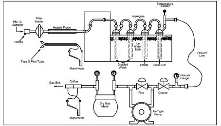
2.1 Sampling Train.

A schematic of the Method 201A sampling train is shown in Figure 1. With the exception of the PM10 sizing device and in-stack filter, this train is the same as an EPA Method 17 train.

Figure 1. Method 201A Sampling Train

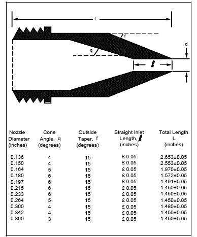
2.1.1 Nozzle. Stainless steel (316 or equivalent) with a sharp tapered leading edge. Eleven nozzles that meet the design specifications in Figure 2 are recommended. A large number of nozzles with small nozzle increments increase the likelihood that a single nozzle can be used for the entire traverse. If the nozzles do not meet the design specifications in Figure 2, then the nozzles must meet the criteria in Section 5.2.

2.1.2 PM10 Sizer. Stainless steel (316 or equivalent), capable of determining the PM10 fraction. The sizing device shall be either a cyclone that meets the specifications in Section 5.2 or a cascade impactor that has been calibrated using the procedure in Section 5.4.

2.1.3 Filter Holder. 63-mm, stainless steel. An Andersen filter, part number SE274, has been found to be acceptable for the in-stack filter.

NOTE: Mention of trade names or specific products does not constitute endorsement by the Environmental Protection Agency.

2.1.4 Pitot Tube. Same as in Method 5, Section 2.1.3. The pitot lines shall be made of heat resistant tubing and attached to the probe with stainless steel fittings.

2.1.5 Probe Liner. Optional, same as in Method 5, Section 2.1.2.

2.1.6 Differential Pressure Gauge, Condenser, Metering System, Barometer, and Gas Density Determination Equipment. Same as in Method 5, Sections 2.1.4, and 2.1.7 through 2.1.10, respectively.

2.2 Sample Recovery.

2.2.1 Nozzle, Sizing Device, Probe, and Filter Holder Brushes. Nylon bristle brushes with stainless steel wire shafts and handles, properly sized and shaped for cleaning the nozzle, sizing device, probe or probe liner, and filter holders.

Figure 2. Nozzle Design Specification

2.2.2 Wash Bottles, Glass Sample Storage Containers, Petri Dishes, Graduated Cylinder and Balance, Plastic Storage Containers, Funnel and Rubber Policeman, and Funnel. Same as in Method 5, Sections 2.2.2 through 2.2.8, respectively.

2.3 Analysis.

Same as in Method 5, Section 2.3.

3. Reagents

The reagents for sampling, sample recovery, and analysis are the same as that specified in Method 5, Sections 3.1, 3.2, and 3.3, respectively.

4. Procedure

4.1 Sampling.

The complexity of this method is such that, in order to obtain reliable results, testers should be trained and experienced with the test procedures.

4.1.1 Pretest Preparation.

Same as in Method 5, Section 4.1.1.

4.1.2 Preliminary Determinations.

Same as in Method 5, Section 4.1.2, except use the directions on nozzle size selection and sampling time in this method. Use of any nozzle greater that 0.16 in. in diameter require a sampling port diameter of 6 inches. Also, the required maximum number of traverse points at any location shall be 12.

4.1.2.1 The sizing device must be in-stack or maintained at stack temperature during sampling. The blockage effect of the CSR sampling assembly will be minimal if the cross-sectional area of the sampling assemble is 3 percent or less of the cross-sectional area of the duct. If the cross-sectional area of the assembly is greater than 3 percent of the cross-sectional area of the duct, then either determine the pitot coefficient at sampling conditions or use a standard pitot with a known coefficient in a configuration with the CSR sampling assembly such that flow disturbances are minimized.

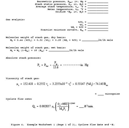
4.1.2.2 The setup calculations can be performed by using the following procedures.

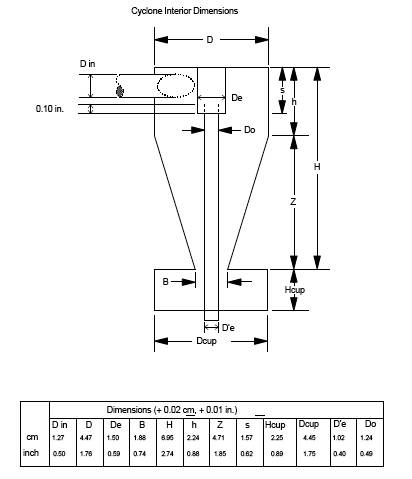
4.1.2.2.1 In order to maintain a cut size of 10 µm in the sizing device, the flow rate through the sizing device must be maintained at a constant, discrete value during the run. If the sizing device is a cyclone that meets the design specifications in Figure 3, use the equations in Figure 4 to calculate three orifice heads (•H): one at the average stack temperature, and the other two at temperatures ±28˚C (±50˚F) of the average stack temperature. Use the •H calculated at the average stack temperature as the pressure head for the sample flow rate as long as the stack temperature during the run is within 28˚C (50˚F) of the average stack temperature. If the stack temperature varies by more than 28˚C (50˚F), then use the appropriate •H.

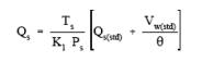
4.1.2.2.2 If the sizing device is a cyclone that does not meet the design specifications in Figure 3, use the equations in Figure 4, except use the procedures in Section 5.3 to determine QS , the correct cyclone flow rate for a 10 µm cut size.

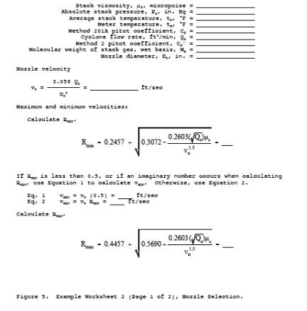
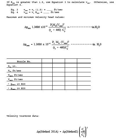
4.1.2.2.3 To select a nozzle, use the equations in Figure 5 to calculate •pmin and •pmax for each nozzle at all three temperatures. If the sizing device is a cyclone that does not meet the design specifications in Figure 3, the example worksheets can be used.

4.1.2.2.4 Correct the Method 2 pitot readings to Method 201A pitot readings by multiplying the Method 2 pitot readings by the square of a ratio of the Method 201A pitot coefficient to the Method 2 pitot coefficient.

Figure 3. Cyclone Design Specifications

Select the nozzle for which •pmin and •pmax bracket all of the corrected Method 2 pitot readings. If more than one nozzle meets this requirement, select the nozzle giving the greatest symmetry. Note that if the expected pitot reading for one or more points is near a limit for a chosen nozzle, it may be outside the limits at the time of the run.

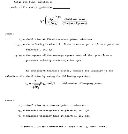
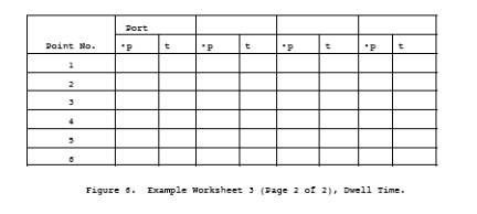
4.1.2.2.5 Vary the dwell time, or sampling time, at each traverse point proportionately with the point velocity. Use the equations in Figure 6 to calculate the dwell time at the first point and at each subsequent point. It is recommended that the number of minutes sampled at each point be rounded to the nearest 15 seconds.

4.1.3 Preparation of Collection Train.

Same as in Method 5, Section 4.1.3, except omit directions about a glass cyclone.

4.1.4 Leak-Check Procedure.

The sizing device is removed before the post-test leak-check to prevent any disturbance of the collected sample prior to analysis.

4.1.4.1 Pretest Leak-Check. A pretest leak-check of the entire sampling train, including the sizing device, is required. Use the leak-check procedure in Method 5, Section 4.1.4.1 to conduct a pretest leak-check.

4.1.4.2 Leak-Checks During Sample Run. Same as in Method 5, Section 4.1.4.1.

4.1.4.3 Post-Test Leak-Check. A leak-check is required at the conclusion of each sampling run. Remove the cyclone before the leak-check to prevent the vacuum created by the cooling of the probe from disturbing the collected sample and use the procedure in Method 5, Section 4.1.4.3 to conduct a post-test leak-check.

4.1.5 Method 201A Train Operation.

Same as in Method 5, Section 4.1.5, except use the procedures in this section for isokinetic sampling and flow rate adjustment. Maintain the flow rate calculated in Section 4.1.2.2.1 throughout the run provided the stack temperature is within 28˚C (50˚F) of the temperature used to calculate •H. If stack temperatures vary by more than 28˚C (50˚F), use the appropriate •H value calculated in Section 4.1.2.2.1. Calculate the dwell time at each traverse point as in Figure 6.

4.1.6 Calculation of Percent Isokinetic Rate and Aerodynamic Cut Size (D50 ).

Calculate percent isokinetic rate and D50 (see Calculations, Section 6) to determine whether the test was valid or another test run should be made. If there was difficulty in maintaining isokinetic sampling rates within the prescribed range, or if the D50 is not in its proper range because of source conditions, the Administrator may be consulted for possible variance.

4.2 Sample Recovery.

If a cascade impactor is used, use the manufacturer's recommended procedures for sample recovery. If a cyclone is used, use the same sample recovery as that in Method 5, Section 4.2, except an increased number of sample recovery containers is required.

4.2.1 Container Number 1 (In-Stack Filter). The recovery shall be the same as that for Container Number 1 in Method 5, Section 4.2.

4.2.3 Container Number 2 (Cyclone or Large PM Catch). This step is optional. The anisokinetic error for the cyclone PM is theoretically larger than the error for the PM10 catch. Therefore, adding all the fractions to get a total PM catch is not as accurate as Method 5 or Method 201. Disassemble the cyclone and remove the nozzle to recover the large PM catch. Quantitatively recover the PM from the interior surfaces of the nozzle and cyclone, excluding the "turn around" cup and the interior surfaces of the exit tube. The recovery shall be the same as that for Container Number 2 in Method 5, Section 4.2.

4.2.4 Container Number 3 (PM10). Quantitatively recover the PM from all of the surfaces from the cyclone exit to the front half of the in-stack filter holder, including the "turn around" cup inside the cyclone and the interior surfaces of the exit tube. The recovery shall be the same as that for Container Number 2 in Method 5, Section 4.2.

4.2.6 Container Number 4 (Silica Gel). The recovery shall be the same as that for Container Number 3 in Method 5, Section 4.2.

4.2.7 Impinger Water. Same as in Method 5, Section 4.2, under "Impinger Water."

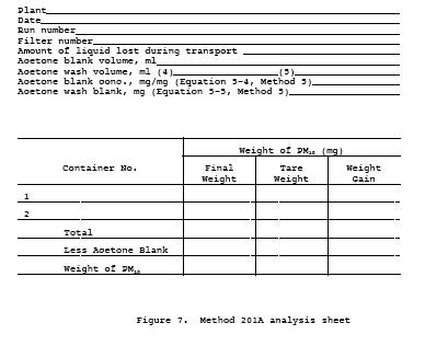
4.3 Analysis.

Same as in Method 5, Section 4.3, except handle Method 201A Container Number 1 like Container Number 1, Method 201A Container Numbers 2 and 3 like Container Number 2, and Method 201A Container Number 4 like Container Number 3. Use Figure 7 to record the weights of PM collected. Use Figure 5-3 in Method 5, Section 4.3, to record the volume of water collected.

4.4 Quality Control Procedures.

Same as in Method 5, Section 4.4.

5. Calibration

Maintain an accurate laboratory log of all calibrations.

5.1 Probe Nozzle, Pitot Tube, Metering System, Probe Heater Calibration, Temperature Gauges, Leak-check of Metering System, and Barometer.

Same as in Method 5, Section 5.1 through 5.7, respectively.

5.2 Probe Cyclone and Nozzle Combinations.

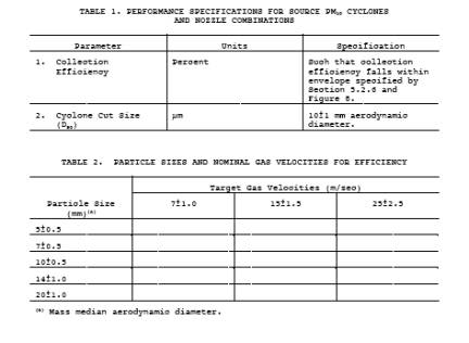
The probe cyclone and nozzle combinations need not be calibrated if both meet design specifications in Figures 2 and 3. If the nozzles do not meet design specifications, then test the cyclone and nozzle combinations for conformity with performance specifications (PS's) in Table 1. If the cyclone does not meet design specifications, then the cyclone and nozzle combination shall conform to the PS's and calibrate the cyclone to determine the relationship between flow rate, gas viscosity, and gas density. Use the procedures in Section 5.2 to conduct PS tests and the procedures in Section 5.3 to calibrate the cyclone. The purpose of the PS tests are to confirm that the cyclone and nozzle combination has the desired sharpness of cut. Conduct the PS tests in a wind tunnel described in Section 5.2.1 and particle generation system described in Section 5.2.2. Use five particle sizes and three wind velocities as listed in Table 2. A minimum of three replicate measurements of collection efficiency shall be performed for each of the 15 conditions listed, for a minimum of 45 measurements.

5.2.1 Wind Tunnel. Perform the calibration and PS tests in a wind tunnel (or equivalent test apparatus) capable of establishing and maintaining the required gas stream velocities within 10 percent.

5.2.2 Particle Generation System. The particle generation system shall be capable of producing solid mono-dispersed dye particles with the mass median aerodynamic diameters specified in Table 2. Perform the particle size distribution verification on an integrated sample obtained during the sampling period of each test. An acceptable alternative is to verify the size distribution of samples obtained before and after each test, with both samples required to meet the diameter and mono-dispersity requirements for an acceptable test run.

5.2.2.1 Establish the size of the solid dye particles delivered to the test section of the wind tunnel by using the operating parameters of the particle generation system, and verify them during the tests by microscopic examination of samples of the particles collected on a membrane filter. The particle size, as established by the operating parameters of the generation system, shall be within the tolerance specified in Table 2. The precision of the particle size verification technique shall be at least ±0.5 µm, and particle size determined by the verification technique shall not differ by more than 10 percent from that established by the operating parameters of the particle generation system.

5.2.2.2. Certify the mono-dispersity of the particles for each test either by microscopic inspection of collected particles on filters or by other suitable monitoring techniques such as an optical particle counter followed by a multi-channel pulse height analyzer. If the proportion of multiplets and satellites in an aerosol; exceeds 10 percent by mass, the particle generation system is unacceptable for the purpose of this test. Multiplets are particles that are agglomerated, and satellites are particles that are smaller than the specified size range.

5.2.3 Schematic Drawings. Schematic drawings of the wind tunnel and blower system and other information showing complete procedural details of the test atmosphere generation, verification, and delivery techniques shall be furnished with calibration data to the reviewing agency.

5.2.4 Flow Measurements. Measure the cyclone air flow rates with a dry gas meter and a stopwatch, or a calibrated orifice system capable of measuring flow rates to within 2 percent.

5.2.5 Performance Specification Procedure. Establish test particle generator operation and verify particle size microscopically. If mono-dispersity is to be verified by measurements at the beginning and the end of the run rather than by an integrated sample, these measurements may be made at this time.

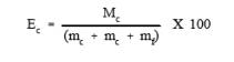
5.2.5.1 The cyclone cut size, or D50, of a cyclone is defined here as the particle size having a 50 percent probability of penetration. Determine the cyclone flow rate at which D50 is 10 µm. A suggested procedure is to vary the cyclone flow rate while keeping a constant particle size of 10 µm. Measure the PM collected in the cyclone (mc), the exit tube (mt), and the filter (mf). Calculate cyclone efficiency (Ec) for each flow rate as follows:

5.2.5.2 Do three replicates and calculate the average cyclone efficiency [Ec(avg)] as follows:

where E1, E2, and E3 are replicate measurements of Ec

5.2.5.3 Calculate the standard deviation (•) for the replicate measurements of Ec as follows:

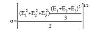
If • exceeds 0.10, repeat the replicated runs.

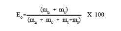
5.2.5.4 Measure the overall efficiency of the cyclone and nozzle, Eo at the particle sizes and nominal gas velocities in Table 2 using the following procedure.

5.2.5.5 Set the air velocity and particle size from one of the conditions in Table 2. Establish isokinetic sampling conditions and the correct flow rate in the cyclone (obtained by procedures in this section) such that the D50 is 10 µm. Sample long enough to obtain ±5 percent precision on total collected mass as determined by the precision and the sensitivity of measuring technique. Determine separately the nozzle catch (mn), cyclone catch (mc), cyclone exit tube (Mt), and collection filter catch (mf) for each particle size and nominal gas velocity in Table 2. Calculate overall efficiency (Eo) as follows:

5.2.5.6 Do three replicates for each combination of gas velocity and particle size in Table 2. Use the equation below to calculate the average overall efficiency [Eo(avg)] for each combination following the procedures described in this section for determining efficiency.

where E1, E2, and E3 are replicate measurements of Eo

5.2.5.7 Use the formula in Section 5.2.5.3 to calculate • for the replicate measurements. If • exceeds 0.10 or if the particle sizes and nominal gas velocities are not within the limits specified in Table 2, repeat the replicate runs.

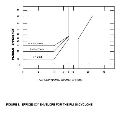
5.2.6 Criteria for Acceptance. For each of the three gas stream velocities, plot the Eo(avg) as a function of particle size on Figure 8. Draw smooth curves through all particle sizes. Eo(avg) shall be within the banded region for all sizes, and the Ec(avg) shall be 50 ± 0.5 percent at 10 µm.

5.3 Cyclone Calibration Procedure.

The purpose of this procedure is to develop the relationship between flow rate, gas viscosity, gas density, and D50.

5.3.1 Calculate Cyclone Flow Rate. Determine flow rates and D50 's for three different particle sizes between 5 µm and 15 µm, one of which shall be 10 µm. All sizes must be determined within 0.5 µm. For each size, use a different temperature within 60˚C (108˚F) of the temperature at which the cyclone is to be used and conduct triplicate runs. A suggested procedure is to keep the particle size constant and vary the flow rate.

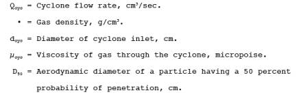
5.3.1.1 On log-log graph paper, plot the Reynolds number (Re) on the abscissa, and the square root of the Stokes 50 number [(Stk50)1/2] on the ordinate for each temperature. Use the following equations to compute both values:

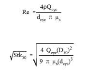
where:

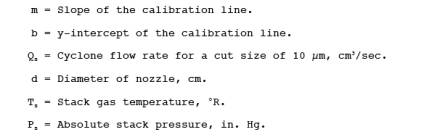
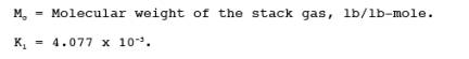
5.3.1.2 Use a linear regression analysis to determine the slope (m) and the Y-intercept (b). Use the following formula to determine Q, the cyclone flow rate required for a cut size of 10 µm.

where:

5.3.1.3 Refer to the Method 201A operators manual, entitled Application Guide for Source PM10 Measurement with Constant Sampling Rate, for directions in the use of this equation for Q in the setup calculations.

5.4 Cascade Impactor.

The purpose of calibrating a cascade impactor is to determine the empirical constant (Stk50), which is specific to the impactor and which permits the accurate determination of the cut sizes of the impactor stages at field conditions. It is not necessary to calibrate each individual impactor. Once an impactor has been calibrated, the calibration data can be applied to other impactors of identical design.

5.4.1 Wind Tunnel. Same as in Section 5.2.1.

5.4.2 Particle Generation System. Same as in Section 5.2.2.

5.4.3 Hardware Configuration for Calibrations. An impaction stage constrains an aerosol to form circular or rectangular jets, which are directed toward a suitable substrate where the larger aerosol particles are collected. For calibration purposes, three stages of the cascade impactor shall be discussed and designated calibration stages 1, 2, and 3. The first calibration stage consists of the collection substrate of an impaction stage and all upstream surfaces up to and including the nozzle. This may include other preceding impactor stages. The second and third calibration stages consist of each respective collection substrate and all upstream surfaces up to but excluding the collection substrate of the preceding calibration stage. This may include intervening impactor stages which are not designated as calibration stages. The cut size, or D50, of the adjacent calibration stages shall differ by a factor of not less than 1.5 and not more than 2.0. For example, if the first calibration stage has a D50 of 12 µm, then the D50 of the downstream stage shall be between 6 and 8 µm.

5.4.3.1 It is expected, but not necessary, that the complete hardware assembly will be used in each of the sampling runs of the calibration and performance determinations. Only the first calibration stage must be tested under isokinetic sampling conditions. The second and third calibration stages must be calibrated with the collection substrate of the preceding calibration stage in place, so that gas flow patterns existing in field operation will be simulated.

5.4.3.2 Each of the PM10 stages should be calibrated with the type of collection substrate, viscid material (such as grease) or glass fiber, used in PM10 measurements. Note that most materials used as substrates at elevated temperatures are not viscid at normal laboratory conditions. The substrate material used for calibrations should minimize particle bounce, yet be viscous enough to withstand erosion or deformation by the impactor jets and not interfere with the procedure for measuring the collected PM.

5.4.4 Calibration Procedure. Establish test particle generator operation and verify particle size microscopically. If mono-dispersity is to be verified by measurements at the beginning and the end of the run rather than by an integrated sample, these measurements shall be made at this time. Measure in triplicate the PM collected by the calibration stage (m) and the PM on all surfaces downstream of the respective calibration stage (m') for all of the flow rates and particle size combinations shown in Table 2. Techniques of mass measurement may include the use of a dye and spectrophotometer. Particles on the upstream side of a jet plate shall be included with the substrate downstream, except agglomerates of particles, which shall be included with the preceding or upstream substrate. Use the following formula to calculate the collection efficiency (E) for each stage.

5.4.4.1 Use the formula in Section 5.2.5.3 to calculate the standard deviation (•) for the replicate measurements. If • exceeds 0.10, repeat the replicate runs.

5.4.4.2 Use the following formula to calculate the average collection efficiency (Eavg ) for each set of replicate measurements.

where E1, E2, and E3 are replicate measurements of E.

5.4.4.3 Use the following formula to calculate Stk for each Eavg.

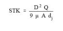
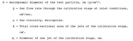
5.4.4.4 Determine Stk50 for each calibration stage by plotting Eavg versus Stk on log-log paper. Stk50 is the Stk number at 50 percent efficiency. Note that particle bounce can cause efficiency to decrease at high values of Stk. Thus, 50 percent efficiency can occur at multiple values of Stk. The calibration data should clearly indicate the value of Stk50 for minimum particle bounce. Impactor efficiency versus Stk with minimal particle bounce is characterized by a monotonically increasing function with constant or increasing slope with increasing Stk.

5.4.4.5 The Stk50 of the first calibration stage can potentially decrease with decreasing nozzle size. Therefore, calibrations should be performed with enough nozzle sizes to provide a measured value within 25 percent of any nozzle size used in PM10 measurements.

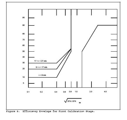
5.4.5 Criteria For Acceptance. Plot Eavg for the first calibration stage versus the square root of the ratio of Stk to Stk50 on Figure 9. Draw a smooth curve through all of the points. The curve shall be within the banded region.

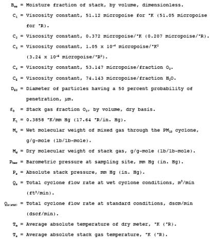
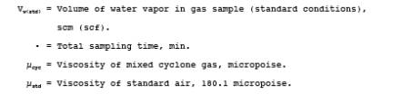
6. Calculations

6.1 Nomenclature.

6.2 Analysis of Cascade Impactor Data. Use the manufacturer's recommended procedures to analyze data from cascade impactors.

6.3 Analysis of Cyclone Data. Use the following procedures to analyze data from a single stage cyclone.

6.3.1 PM Weight. Determine the PM10 catch in the PM10 range from the sum of the weights obtained from Container Numbers 1 and 3 less the acetone blank.

6.3.2 Total PM Weight (optional). Determine the PM catch for greater than PM10 from the weight obtained from Container Number 2 less the acetone blank, and add it to the PM10 weight.

6.3.3 PM10 Fraction. Determine the PM10 fraction of the total particulate weight by dividing the PM10 particulate weight by the total particulate weight.

6.3.4 Aerodynamic Cut Size. Calculate the stack gas viscosity as follows:

6.3.4.1 The PM10 flow rate, at actual cyclone conditions, is calculated as follows:

6.3.4.2 Calculate the molecular weight on a wet basis of the stack gas as follows:

6.3.4.3 Calculate the actual D50 of the cyclone for the given conditions as follows:

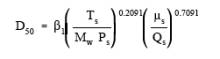
6.3.5 Acceptable Results. The results are acceptable if two conditions are met. The first is that 9.0 µm ≤ D50 ≤ 11.0 µm. The second is that no sampling points are outside •pmin and •pmax, or that 80 percent ≤ I ≤ 120 percent and no more than one sampling point is outside •pmin and •pmax. If D50 is less than 9.0 µm, reject the results and repeat the test.

7. Bibliography

1. Same as Bibliography in Method 5.

2. McCain, J.D., J.W. Ragland, and A.D. Williamson. Recommended Methodology for the Determination of Particle Size Distributions in Ducted Sources, Final Report. Prepared for the California Air Resources Board by Southern Research Institute. May 1986.

3. Farthing, W.E., S.S. Dawes, A.D. Williamson, J.D. McCain, R.S. Martin, and J.W. Ragland. Development of Sampling Methods for Source PM10 Emissions. Southern Research Institute for the Environmental Protection Agency. April 1989. NTIS PB 89 190375, EPA/600/3-88-056.

4. Application Guide for Source PM10 Measurement with Constant Sampling Rate, EPA/600/3-88-057.